Typically, you would begin a miRNA expression analysis with the same steps outlined in the Importing Affymetrix CEL files section of the Gene Expression tutorial. Here, the data has already been imported and attributes added. 

To being our analysis, we will open the miRNA Expression workflow. 

• Select the miRNA Expression workflow from the Workflows drop-down menu

The miRNA Expression workflow provides a series of steps for analyzing miRNA expression data and integrating it with gene expression data (Figure 1).

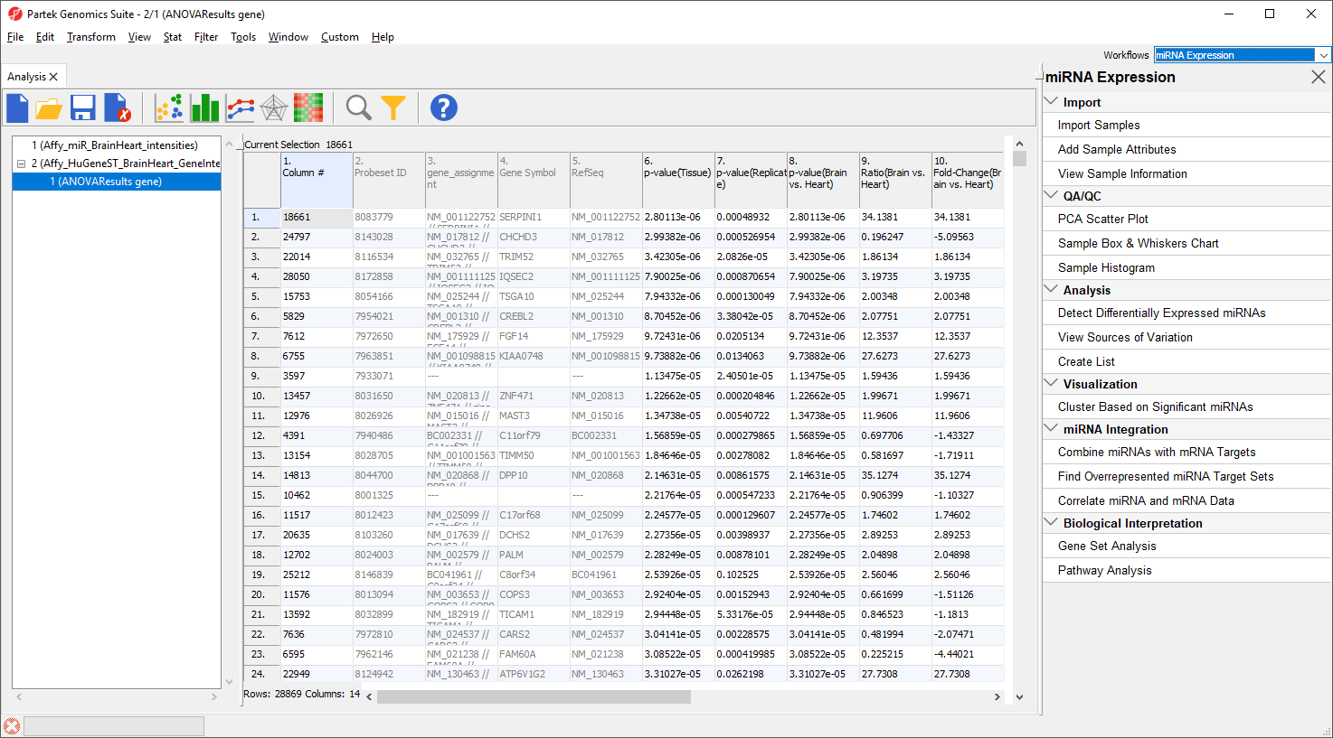
Figure 1. The miRNA Expression workflow

Exploratory data analysis

Principal Components Analysis (PCA) is an excellent method to visualize similarities and differences between the samples in a data set. PCA can be invoked through a workflow, by selecting  from the main command bar, or by selecting Scatter Plot from the View section of the main toolbar. We will use a workflow. 

• Select the Affy_miR_BrainHeart_intensities spreadsheet

This is the probe intensities spreadsheet for the miRNA expression data (Figure 2). Each row is a sample; columns 7 to 9 give attribute information about each sample including tissue, replicate number, and scan date, while columns 10 on give prove intensities values. 

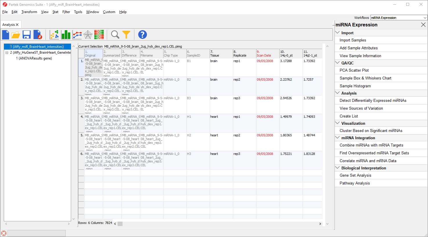
Figure 2. Viewing the miRNA probe intensities spreadsheet

• Select PCA Scatter Plot from the QA/QC section of the workflow

A new tab will open showing a PCA scatter plot (Figure 3).

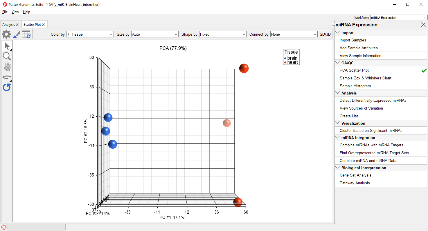
Figure 3. PCA scatter plot. Samples are spheres. Samples with more similar miRNA expression are close together while dissimilar samples are further apart.

In this PCA scatter plot, each point represents a sample in the spreadsheet. Points that are close together in the plot are more similar, while points that are far apart in the plot are more dissimilar. 

To better view the data, we can rotate the plot.

• Select () to activate Rotate Mode
• Click and drag to rotate the plot 

Rotating the plot allows us to look for outliers in the data on each of the three principal components (PC1-3). The percentage of the total variation explained by each PC is listed by its axis label. The chart label shows the sum percentage of the total variation explained by the displayed PCs. 

Here, we can see that the brain and heart samples are well separated across PC1, which is expected. 

For more information about customizing the plot, please see Exploring the data set with PCA from the Gene Expression with Batch Effect tutorial. 

Detecting differentially expressed miRNAs

Next, we will identify miRNAs that are differentially expressed between brain and heart tissues. 

• Select the Analysis tab
• Select the Affy_miR_BrainHeart_intensities spreadsheet
• Select Detect Differentially Expressed miRNAs from the Analysis section of the workflow

The ANOVA dialog (Figure 4) allows us to configure the comparisons we want to make between samples and groups within the data set. 

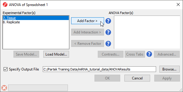
Figure 4. ANOVA dialog

• Select Tissue from the Experimental Factor(s) panel 
• Select Add Factor > to move Tissue to the ANOVA Factor(s) panel

The Contrasts... button will now be available to select. 

• Select Contrasts... 

The Configure ANOVA dialog (Figure 5) is used to set up contrasts. Contrasts are the comparisons between groups and are where experimental questions can be asked. In this study, we are asking what miRNAs are differentially expressed between heart and brain tissue. 

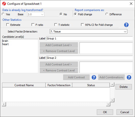
Figure 5. ANOVA configuration dialog

• Select Yes for Data is already log transformed?
• Select Fold change for Report comparisons as
• Select 7. Tissue from the Select Factor/Interaction drop-down menu
• Select brain from the left panel 
• Select Add Contrast Level > to move brain to the upper group - initially Group 1
• Select heart from the left panel
• Select Add Contrast Level > to move heart to the lower group - initially Group 2

This contrast (Figure 6) will compare expression of miRNAs in brain samples to expression in heart samples with brain as the numerator and heart as the denominator for fold-change calculations. 

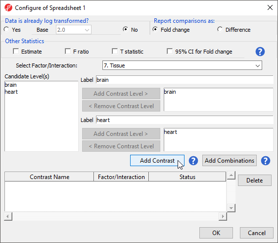
Figure 6. Configuring a contrast between brain and heart tissue in the ANOVA dialog

• Select Add Contrast 
• Select OK 

The Contrasts... button should now read Contrasts Included. 

• Select OK to run the ANOVA as configured

An ANOVA Results sheet, ANOVAResults, will be created as a child spreadsheet of Affy_miR_BrainHeart_intensities (Figure 7). In this spreadsheet, each row represents a probe set and the columns represent the computation results for that probe set. Although not synonymous, probe set and gene will be treated as synonyms in this tutorial for convenience. By default, the genes are sorted in ascending order by the p-value of the first categorical factor, which, in this case, is Tissue. This means the most significant differentially expressed miRNAs between the brain and heart (up-regulated and donw-regulated) are at the top of the spreadsheet. 

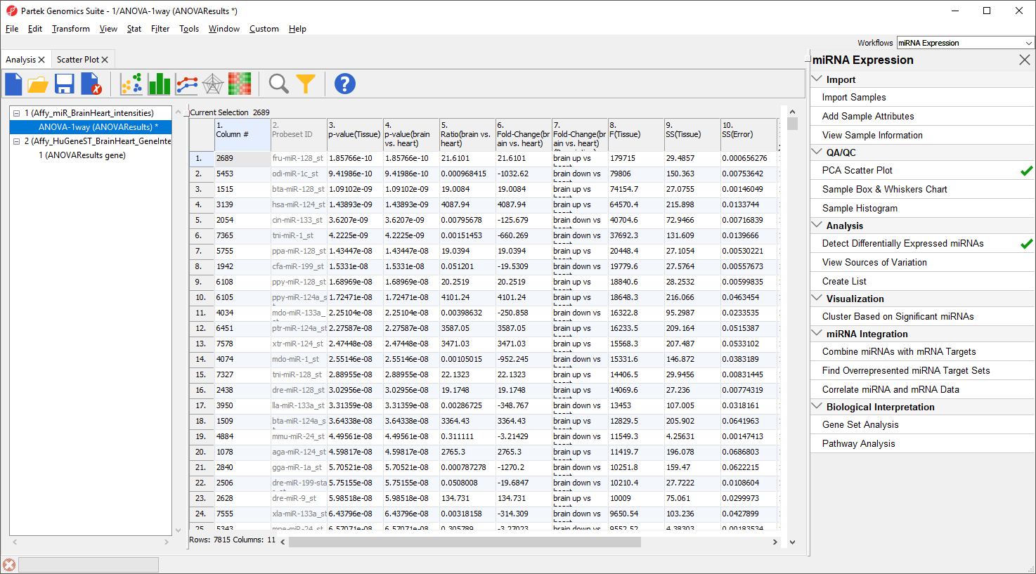
Figure 7. Viewing the ANOVA results spreadsheet

You may explore what is known about any listed miRNA using external databases TargetScan, miRBase, microRNA.org, or miR2Disease, by right-clicking a row header, selecting Find miRNA in... and choosing one of the external databases. This will open a web page in your default web browser and requires your computer be connected to the internet. 

For more information about AVOVA in Partek Genomics Suite, see Identifying differentially expressed genes using ANOVA. 

Creating a list of miRNAs of interest

The ANOVA results spreadsheet includes every miRNA on the array for a total of 7815 miRNAs. However, many of these miRNAs are not significantly differentially expressed between brain and heart and, thus, are not of interest. Next, we will create a filtered list of significantly differentially expressed miRNAs.

• Select the ANOVAResults spreadsheet
• Select Create List from the Analysis section of the workflow

The List Manager dialog will open (Figure 8). 

• Select brain vs. heart under Contrast: find genes that change between two categories

By default, the fold-change and significance thresholds are set to > 2, < -2 and p-value with FDR < 0.05. These defaults are appropriate for this tutorial so we will leave them in place.

• Select Create to create a new list, brain vs. heart containing only the 1404 miRNAs that pass the criteria 

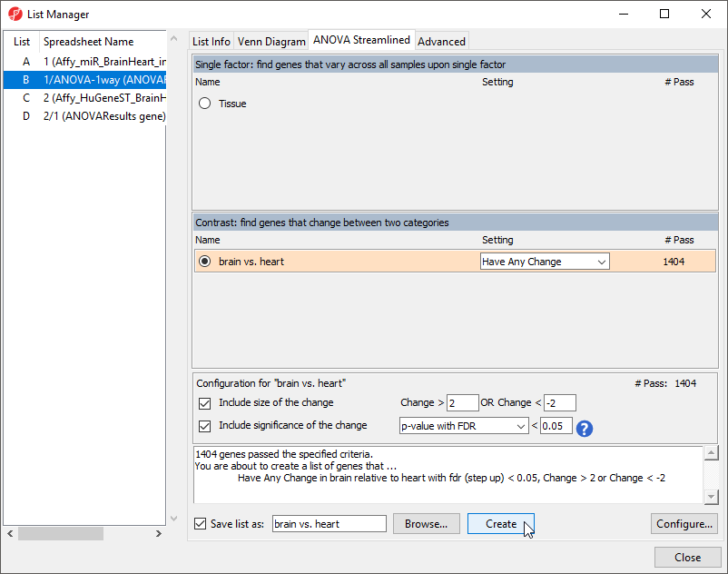
Figure 8. Creating a list of significantly differentially expressed miRNAs

A new spreadsheet, brain vs. heart will be created as a child spreadsheet of Affy_miR_BrainHeart (Figure 9).

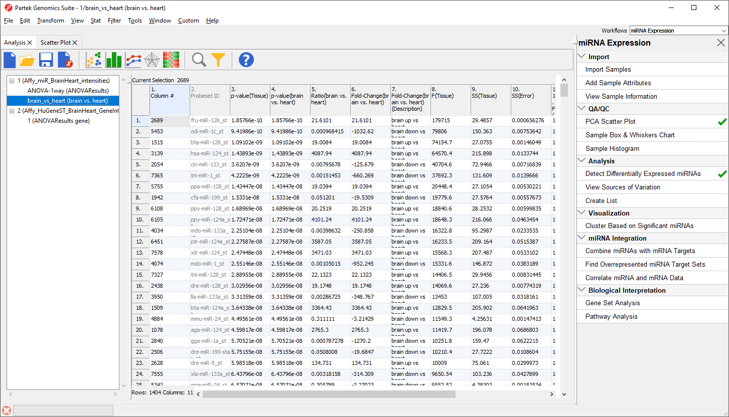
Figure 9. Viewing brain vs. heart spreadsheet

To view the miRNAs with the largest difference between tissues, we can sort by fold-change.

• Right-click the 6. Fold-Change(brain vs. heart) column header
• Select Sort Descending by Absolute Value from the pop-up menu

The top 33 miRNAs we see (Figure 10) are all miR-124 from different species. The miRNA miR-124 is the most abundant miRNA in neuronal cells so this finding is expected. The multiple species versions of miR-124 are present because Affymetrix GeneChip miRNA arrays provide comprehensive coverage of miRNAs from multiple organisms including human, mouse, rat, canine, monkey, and many more on a single chip. The miRNAs from these different species are highly homologous so probes targeting miRNAs from other species will hybridize with human miRNAs. Therefore, we need to filter the list of miRNAs to include only human miRNAs.

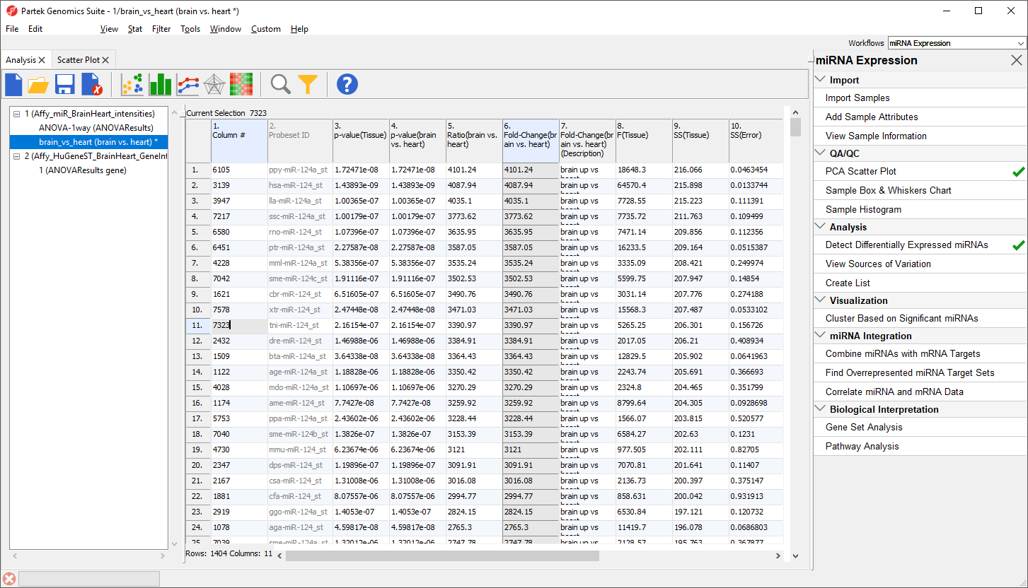
Figure 10. miR-124 is highly differentially expressed in brain vs. heart

To do this, we need to add a new annotation column containing species information for each probe.

• Right-click on the 2. Probeset ID column header
• Select Insert Annotation from the pop-up menu
• Select Add as categorical
• Check Species Scientific Name (Figure 11)
• Select OK to add the annotation column
  
  

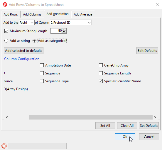
Figure 11. Inserting species annotation column

The table now includes a column 3. Species Scientific Name with the species name of each miRNA. We can now filter to include only human miRNAs.

• Right-click the 3. Species Scientific Name column header
• Select Find / Replace / Select... from the pop-up menu
• Type Homo sapiens for Find What
• Select Only in column for Search
• Select 3. Species Scientific Name from the drop-down menu next to the Only in column option
• Select Select All (Figure 12)
  
  

 

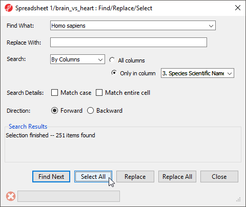
Figure 12. Configuring the Find / / Replace / Select... dialog

The search should find and select 251 miRNAs. 

• Select Close
• Right-click any of the row headers that are selected 
• Select Filter Include from the pop-up menu

The spreadsheet will now include only the 251 miRNAs from human (Figure 13). The first row is still miR-124 with a fold change of 4087.94. The black and gold bar on the right-hand side of the spreadsheet indicates the fraction of rows that have been filtered. To retain this filtered list, we can create a new spreadsheet. 

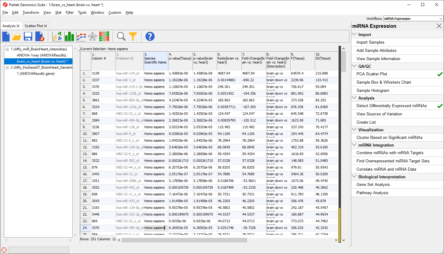
Figure 13. Viewing differentially expressed human miRNAs

• Right-click the brain_vs_heart spreadsheet in the spreadsheet tree
• Select Clone... from the pop-up menu

Cloning a spreadsheet while a filter is applied copies only the included rows/columns. 

• Name the spreadsheet brain_vs_heart_human
• Select Affy_miR_BrainHeart_intensities from the drop-down menu Create new spreadsheet as a child of spreadsheet 
• Select  
• Name the new file brain vs. heart human
• Select Save

The new spreadsheet includes only the 251 human miRNAs that are significantly differentially expressed between brain and heart tissue (Figure 14). 

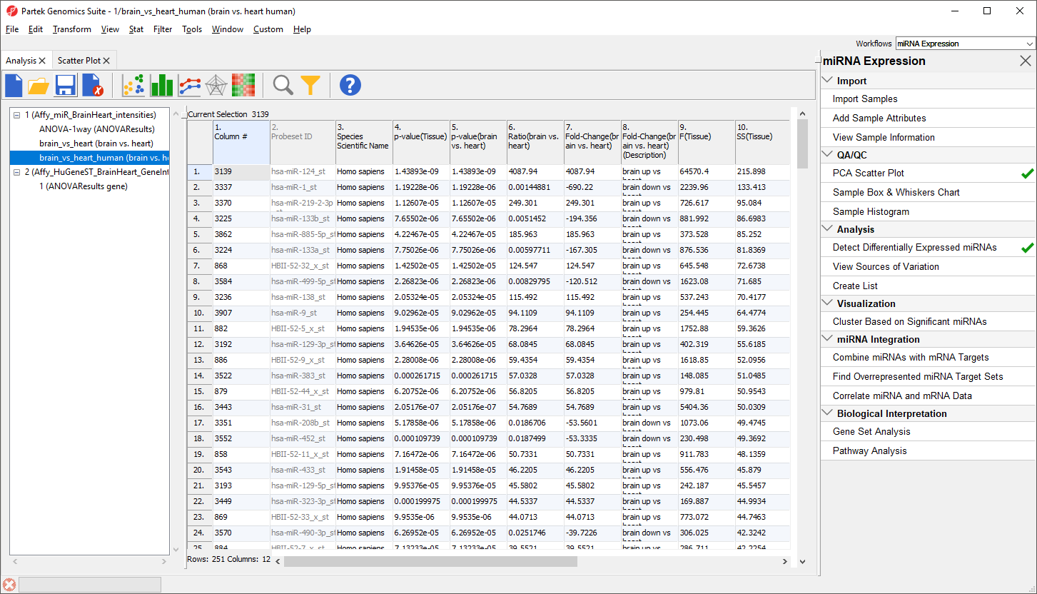
Figure 14. Viewing the filtered human miRNAs spreadsheet

The next step in our analysis will be integrating miRNA and gene expression data.

Your Rating:

Thanks for voting!

Please Wait

Results:

32

rates