In Partek Flow, we use tools from Monocle 3 ⁽¹⁾ to build trajectories, identify states and branch points, and calculate pseudotime values. The output of Trajectory analysis task includes an interactive 2D/3D visualization for viewing the trajectory trees and setting the root states (starting points of the trajectories). From the Trajectory analysis report, you can run a second task, Calculate pseudotime, which adds a numeric cell-level attribute, Pseudotime, calculated using the chosen root states. 

Prerequisites for the Analysis

Trajectory analysis by Monocle 3 requires data normalization and preprocessing. Regarding the normalization, we suggest to first use the Normalization and scaling section of the toolbox to normalize by counts per million (CPM), add offset of 1, and log2 transform. After that, launch the Trajectory analysis on the Normalized counts node.

According to the Monocle 3 authors, you may want to filter in the top 5,000 genes with the highest variance (2,000 genes for datasets with fewer than 5,000 cells, and 300 genes for datasets with fewer than 1,000 cells) ⁽¹⁾. Those numbers should be used as a guidance for the first-pass analysis and may need to be optimized, depending on the project at hand and the biological question.

Setting up Trajectory Analysis

To run Trajectory analysis tool, select the Normalized counts data node (or equivalent) and go to the toolbox: Exploratory analysis > Trajectory analysis

The configuration dialog presents four options (Figure 1).

1. Dimensionality of reduced space. This option specifies the number of UMAP dimensions that the original data are reduced to, in order to learn the trajectory tree (dimensionality of original data equals the number of genes). Default is two, meaning that the trajectory plot will be draw in two dimensions. To get a 3D trajectory plot, increase this option to 3.
2. Scaling. Normalized expression values can be further transformed by scaling to unit variance and zero mean (i.e. converting to Z score). The use of this option is recommended ⁽¹⁾.
3. Data is logged. Select this option if the data have already been log-transformed upstream. When selected, Monocle 3 will skip the log2 step on the input data (see below).
4. Programmatically calculate default root nodes. If not selected, user has to specify the root nodes of the trajectory tree manually (default). Depending on the available meta-data, Monocle 3 may be able to pick the root nodes programmatically (see below for details)

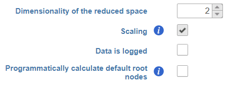
Figure 1. Specifying Monocle 3 default options. If log normalization has been performed in Partek Flow, the Data is logged option will be selected automatically

Under the hood, Monocle 3 will perform log2 transformation of the gene count matrix (if Data is logged was unselected), scale the matrix (if Scaling was selected), and project the gene count matrix into the top 50 principal components. Next, the dimensionality reduction will be implemented by UMAP (using default settings of the reduce dimension command).

Trajectory Analysis Result

Result of running Trajectory analysis in Partek Flow is the Trajectory result data node. Double clicking on the node opens a Data Viewer window with the trajectory plot (Figure 2). Cell trajectory graph shows position of each cell (blue dot) with respect to the UMAP coordinates (axes). Cell trajectories (one or more, depending on the data set) are depicted as black lines. Gray circles are trajectory nodes (i.e. cell communities).

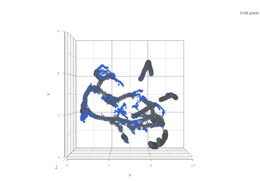
Figure 2. Cell trajectory graph. Blue dots are individual cells (total count is displayed in the upper right). Black line represents the structure of the trajectory graph. Gray circles are nodes or leaves. The axes represent UMAP coordinates.

To show / hide cell trajectory tree and trajectory nodes, select Axes in Configure section and on the upper-right corner of the dialog, select the Extra data drop-down options (Figure 2).

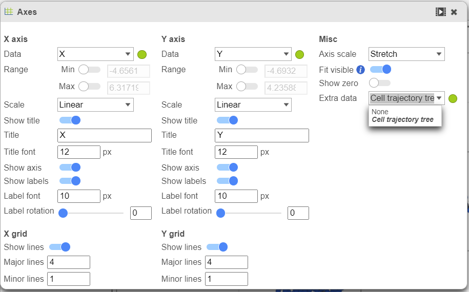
Figure 3. Extra data card enables the user to turn the trajectory tree and the trajectory nodes on or off

Pseudotime Analysis

To perform pseudotime analysis, you need to point to the cells at the beginning of the biological process you are interested in. For example, cells at the earliest stage of differentiation sequence. There are two ways to perform pseudotime analysis in Partek Flow, depending on the way the root nodes (=cells at the beginning of pseudotime) are defined.

1. Manual selection of root node. The user has to specify the root nodes (one or more).
2. Automatic selection of the root node. The root node is picked by the algorithm.

Manual Selection of the Root Node

If you want to manually pick the root nodes, leave the option Programmatically calculate default root nodes unselected when setting up the Trajectory analysis. 

To start, select the root cell nodes (gray circles in trajectory tree) by left-clicking. If the trajectory result consists of more than one trajectory tree, you can specify more than one root node, e.g. one root node per trajectory tree (ctrl & click). If no root node is specified for a tree, that tree will not be included in the pseudotime calculation. Figure 4 shows an example where seven root nodes were identified.

Figure 4. Identification of root nodes for pseudotime analysis. The selected nodes are in dark gray

Once you have identified all the root nodes, click on Additional button in Tools section on the left panel, push the Calculate pseudotime button in the dialog (Figure 5).

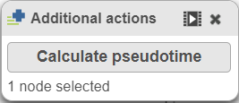
Figure 5. Once the root cell nodes are selected, use the Calculate pseudotime button to start the calculation. In this example, seven root nodes were specified

As a result, the cells will be annotated by pseudotime, using green to red gradient (start and end, respectively) (Figure 6). If, for a particular tree, no root node has been identified, those cells will be omitted from the pseudotime calculation and will be colored in black (Figure 9).

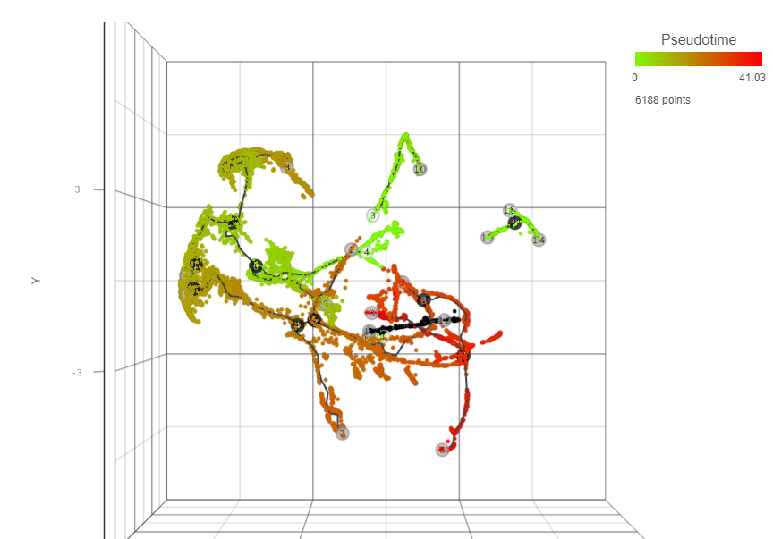
Figure 6. Cells annotated by pseudotime, from start (green) to end (red)

Pseudotime calculation display the structure of the graph using black lines. The circles with numbers (cell nodes) on the black lines represent special points. There are three types of cell nodes:

1. Root node (white). Root nodes are start points of the pseudotime and were defined by the user in the previous step (e.g. node 4 in Figure 7).
2. Branch node (black). Branch nodes indicate where the trajectory tree forks out; i.e. each branch represents a different cell fate or different trajectory (e.g. nodes 3-6, and 8 in Figure 7).
3. Leaf (light gray). Leaves correspond to different cell fates / different trajectory outcomes (e.g. nodes 5, 9, and 12 in Figure 7). The leaves correspond to cell states of Monocle 2.

The numbers within the circles are provided for reference purposes only. The intermediate nodes from the previous step have been removed.

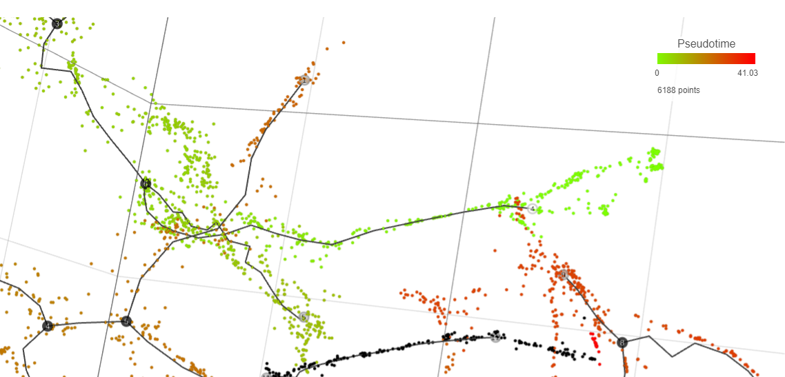
Figure 7. Following pseudotime analysis, three types of nodes can be identified on the trajectory plot. White circles - root nodes (beginning of pseudotime), black circles - branch nodes (splitting of differentiation pathway), and light gray nodes - leaves (outcome of differentiation pathway)

Automatic Selection of the Root Node

If suitable meta-data are available, it is possible to automatically select the root node. For example, you may know which cells were harvested from the earliest time points. The cells need to be annotated by that information (Annotate Cells task) before running Trajectory analysis. The annotation will, in turn, be available in the Trajectory analysis setup dialog, upon selecting the Programmatically calculate default root nodes option (Figure 8).

1. Attribute for root nodes. The drop down list will show the available cell-level attributes. Specify the one which should be used to identify the root nodes. In the example in Figure 8, the attribute embryo.time.bin describes the developmental time point at which the cells were harvested.
2. Attribute value for root nodes. The drop down list will show the content of the attribute selected under Attribute for root nodes. Specify the entry that corresponds to the earliest time point (i.e. beginning of pseuodtime). In the example in Figure 8, the earliest time point was the time bin 130-170.

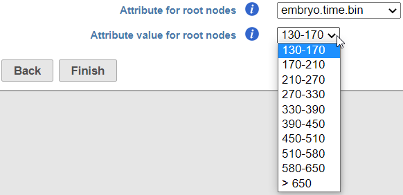
Figure 8. When the option Programmatically select the default root node is turned on, the user can specify the cell attribute which specifies the root node information (Attribute for root nodes) and the level of that attribute corresponding to the earliest pseudotime (Attribute value for root nodes)

Once the options have been set, Monocle 3 will first group the cells according to which trajectory node they are nearest to. It then calculates the fraction of the cells from the earliest time point at each trajectory node. Finally, it picks the node with the highest prevalence of the early cells and treats it as the root node.

In Figure 9, node 1 has been picked as the beginning of pseudotime, due to the high number of cells from the embryo.time.bin 130-170 grouped around that node (a 2D view is shown).

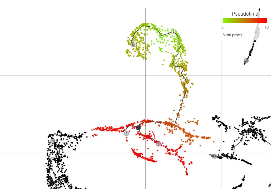
Figure 9. Trajectory tree colored by pseudotime, following automatic selection of the root node (2D view). White circles - root node (beginning of pseudotime), black circles - branch nodes (splitting of differentiation pathway), and light gray nodes - leaves (outcome of differentiation pathway), black dots - cells not connected to the main trajectory tree.

References

1. Cao J, Spielmann M, Qiu X, Huang X, Ibrahim DM, Hill AJ, Zhang F, Mundlos S, Christiansen L, Steemers FJ, Trapnell C, Shendure J. The single-cell transcriptional landscape of mammalian organogenesis. Nature. 2019 Feb;566(7745):496-502. doi: 10.1038/s41586-019-0969-x. Epub 2019 Feb 20. PMID: 30787437; PMCID: PMC6434952.

Your Rating:

Thanks for voting!

Please Wait

Results:

13

rates