Principal components (PC) analysis (PCA) is an exploratory technique that is used to describe the structure of high dimensional data by reducing its dimensionality. It is a linear transformation that converts n original variables (typically: genes or transcripts) into n new variables, which are called PCs, they have three important properties:

• PCs are ordered by the amount of variance explained
• PCs are uncorrelated
• PCs explain all variation in the data

PCA is a principal axis rotation of the original variables that preserves the variation in the data. Therefore, the total variance of the original variables is equal to the total variance of the PCs.

If read quantification (i.e. mapping to a transcript model) was performed by Partek^® E/M algorithm, PCA can be invoked on a quantification output data node (Gene counts or Transcript counts) or, after normalization, on a Normalized counts data node. Select a node on the canvas and then PCA in the Exploratory analysis section of the context sensitive menu.

There are two options for  features contribute (Figure 1):

equally: all the features are standardized to mean of 0 and standard deviation of 1 .  This option will give all the features equal weight in the analysis, this is the default option for e.g bulk RNA-seq data.

by variance: the analysis will give more emphasis to the features with higher variances. This is the default option for e.g. single cell RNA-seq data

If the input data node is in linear scale, you can perform log transformation on PCA calculation. 

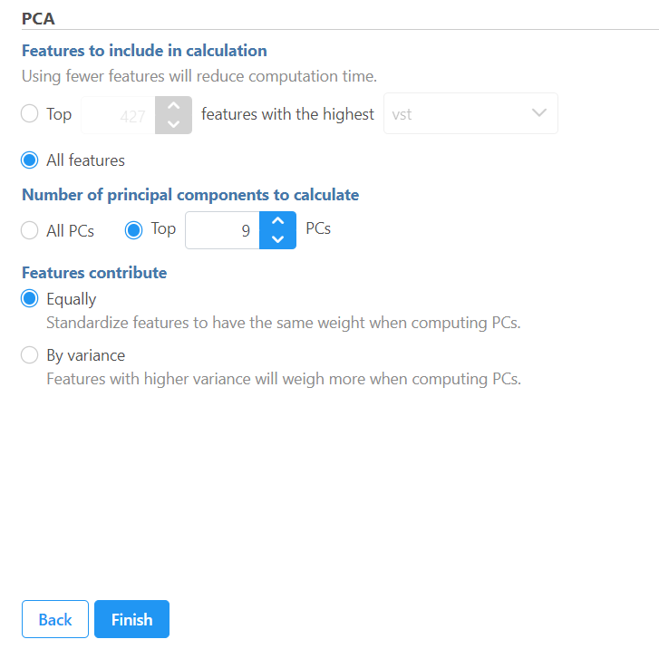
Figure 1. PCA setup dialog

The PCA task creates a new task node, and to open it and see the result, do one of the following: select the PCA task node, proceed to the context sensitive menu and go to the Task result; or double-click on the PCA task node. The report containing eigenvalues, PC projections, component loadings, and mapping error information for the first three PCs. 

When the PCA node is opened in Data viewer, by default, it is the 3D scatterplot, Scree plot with Eigenvalues, and Component loadings table  (Figure 2). Each dot on the 3D scatter plot represents an observation, while the first three PCs are shown on the X-, Y-, and Z-axis respectively, with the information content of an individual PC is in the parenthesis. 

As an exploratory tool, the the PCA scatterplot is applied to view any groupings in the data set and generate hypotheses based on the outcome, or to spot possible outliers.

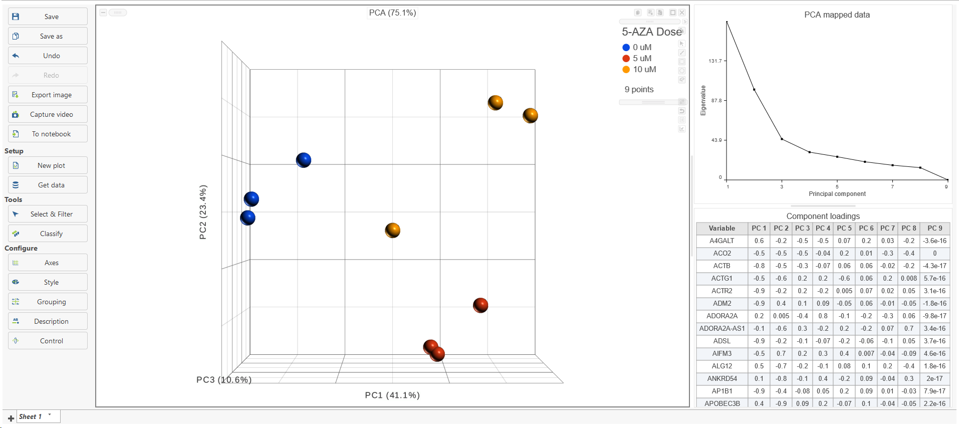
Figure 2. Double-click on the PCA result node to open the Principal components analysis result

To rotate the 3D scatter plot left click & drag. To zoom in or out, use the mouse wheel. Click and drag the legend can move the legend to different location on the viewer.

Detailed configuration on PCA plot can be found by clicking Help>How-to videos>Data viewer section.

In the Data viewer, when a PCA data node is selected from Get Data under Setup (left panel), the node can be dragged and dropped to the screen (Figure 3), then you will have the option to select a scree plot and tables. 

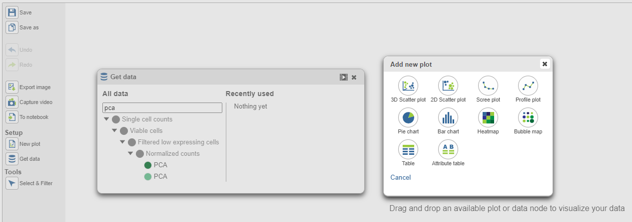
Figure 3. Drag PCA data node to plot

When choose Scree plot icon , it will plot a 2D viewer, X-axis represents PCs, Y-axis represents eigenvalues (Figure 4)

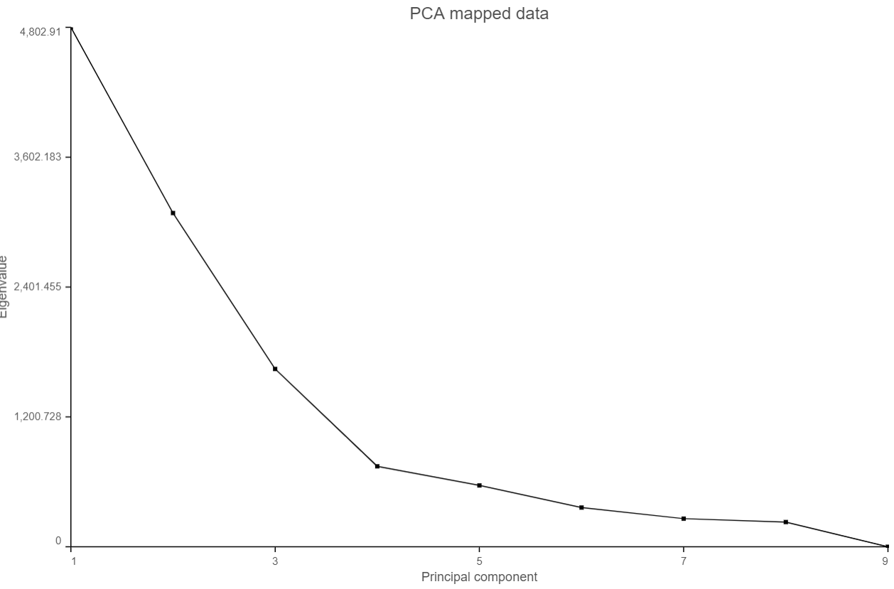
Figure 4. Scree plot

When mouse over on a point on the line, it will display detailed information of the PC. The scree plot shows how much variation each PC represents,  so it is often used to determine the number of principal components to keep for downstream analysis (e.g. tSNE, UMAP, graph-base clustering). The "elbow" point of the graph where the eigenvalues seem to level off should be considered as a cutoff point for downstream analysis.

PCA data node can also be draw as tables, when choose Table icon (), it will display the component loadings matrix in the viewer (Figure 5). The Content can be modified using the Content configuration option; the table can be paged through here or from the lower right corner. 

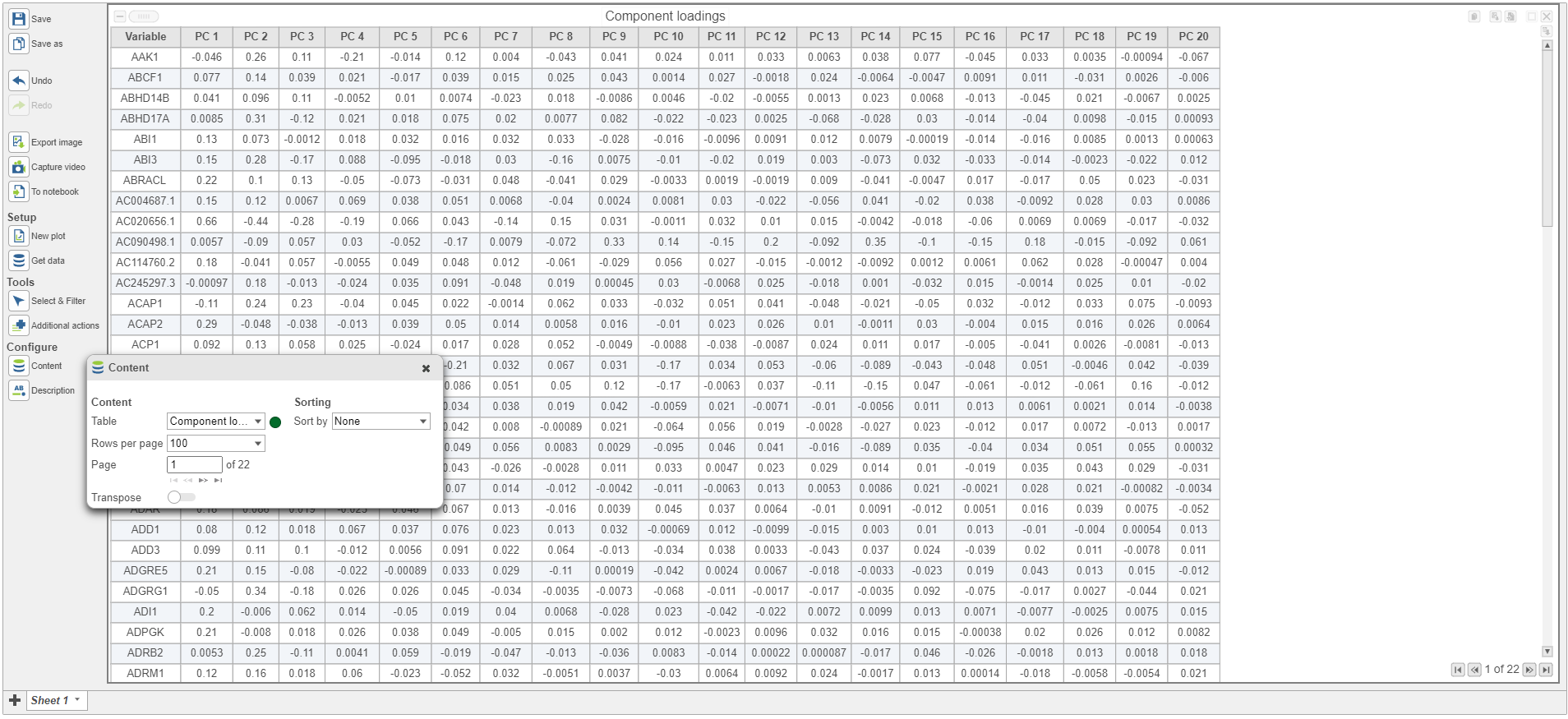
Figure 5. Component loadings are the correlation coefficients between the features and PCs.

In the table, each row is a feature, the column represent PCs, the value is the correlation coefficient. Under Content, there is a PCA projections option,  change to this option to display the projection table (Figure 6). In this table, each row is an observation, each column is a PC, the values are the PC scores. 

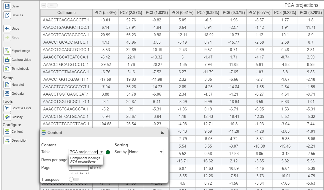
Figure 6. PCA project table

Your Rating:

Thanks for voting!

Please Wait

Results:

37

rates