What is UMAP?

Uniform Manifold Approximation and Projection (UMAP) is a dimensional reduction technique [1]. UMAP aims to preserve the essential high-dimensional structure and present it in a low-dimensional representation. UMAP is particularly useful for visually identifying groups of similar samples or cells in large high-dimensional data sets such as single cell RNA-Seq. 

Running UMAP

We recommend normalizing your data prior to running UMAP, but the task will run on any counts data node. 

• Click the counts data node
• Click the Exploratory analysis section of the toolbox
• Click UMAP
• Click Finish to run

UMAP produces a UMAP task node. Opening the task report launches a scatter plot showing the UMAP results. Each point on the plot is a cell for single cell data or a sample for bulk data. The plot will open in 2D or 3D depending on the user preference.  

UMAP vs. t-SNE

Both t-SNE and UMAP are dimensional reduction techniques that are useful for identifying groups of similar samples in large high-dimensional data sets. A comparison of the techniques for visualizing single cell RNA-Seq data by the authors of UMAP suggests that UMAP runs faster, is more reproducible, gives a more meaningful organization of clusters, and preserves more information about the global structure of the data than t-SNE [2].

In our hands, we find UMAP to be more informative than t-SNE for many data sets. For example, the similarities and differences between clusters are clearly visible with UMAP, but more difficult to judge with t-SNE (Figure 1). 

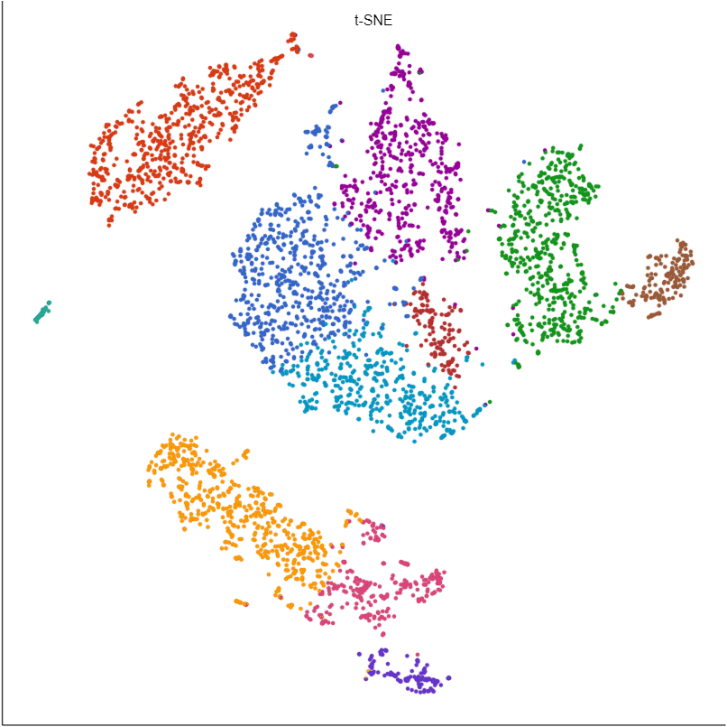
Figure 1. The same data visualized by UMAP (left) and t-SNE (right). Cells in both plots are colored by the same Graph-based clustering results. UMAP clearly shows groups of similar clusters, while t-SNE does not.

Basic UMAP parameters

Initialize output values

Sets the initialization mode. Options are Spectral and Random. 

Spectral - good initial points are chosen using spectral embedding (more accurate)

Random - random initial points are chosen (faster)

Split cells by sample

Chose whether to run UMAP on all samples together or on each sample individually.

Checking the box will run UMAP on each sample individually.

Include features where "Feature type" is 

This option appears when there are multiple feature types in the input data node (e.g., CITE-Seq data). 

Select Any to run on all features or pick a feature type.

Advanced UMAP parameters

Local neighborhood size 

UMAP preserves the local structure of the data by focusing on the distances between each point and its nearest neighbors. Local neighborhood size is the number of nearest neighbors to consider. 

You can adjust this value to prioritize global or local relationships. Smaller values will give a more local view, while larger values will give a more global view (Figure 2). Default is 30.

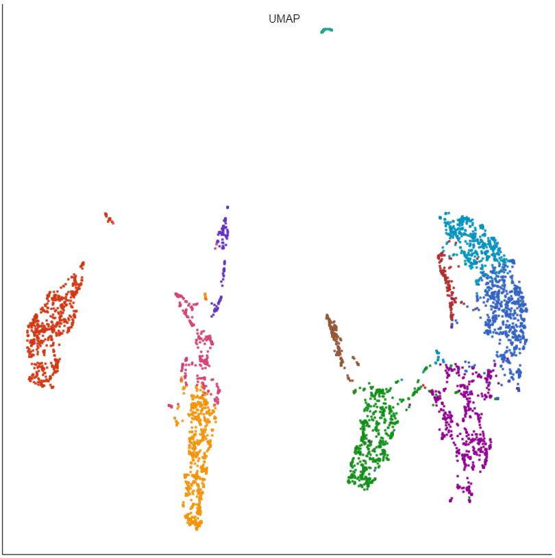
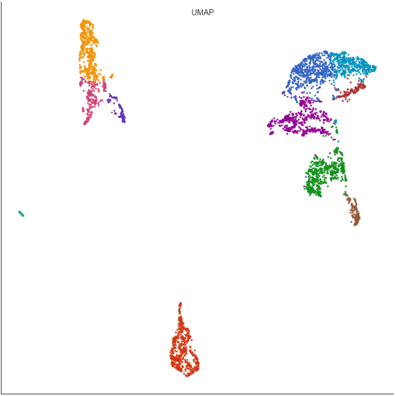
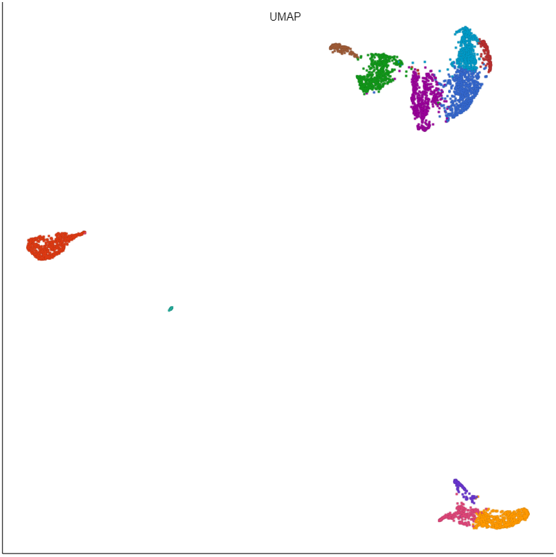
Figure 2. Setting local neighborhood size of UMAP to 5 (left), 15 (middle), 50 (right).

Minimal distance

The effective minimum distance between embedded points. Smaller values will create a more clustered embedding, while larger values will create a more evenly dispersed embedding. 

You can decrease this value to make clusters more tightly packed or increase it to make them looser (Figure 3). Default is 0.3.

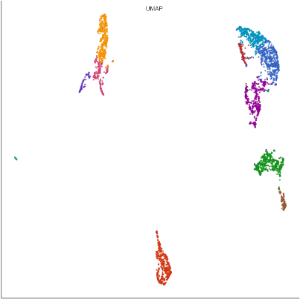
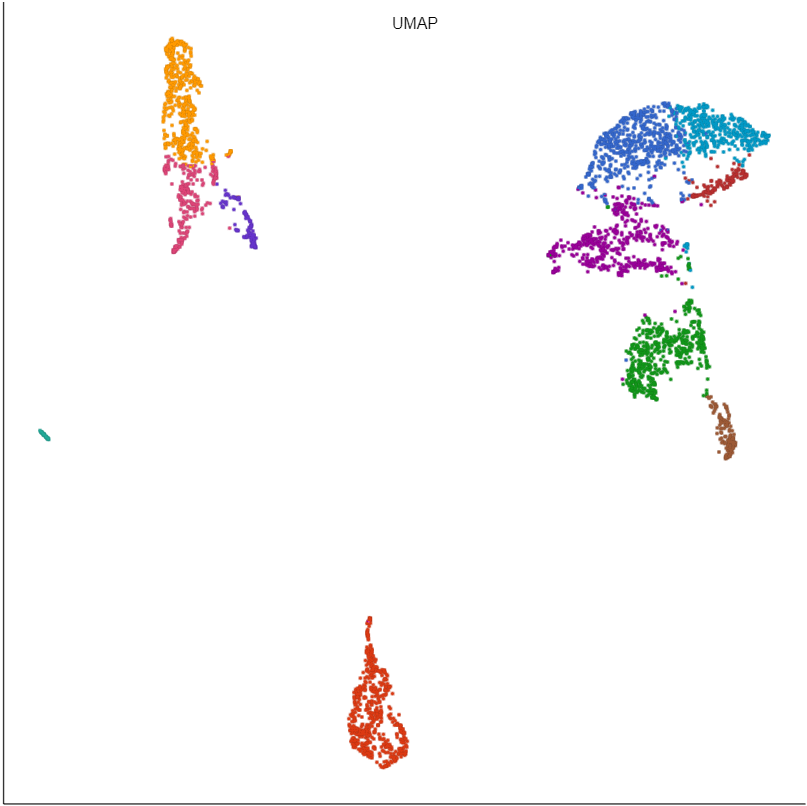
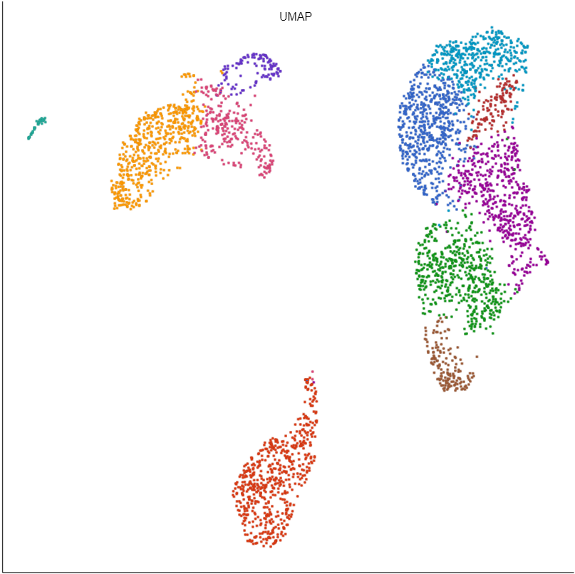
Figure 3. Setting minimal distance of UMAP to 0.02 (left), 0.1 (center), or 0.5 (right)

Distance metric 

The metric to use when computing distances in high-dimensional space. Options are Euclidean, Manhattan, Chebyshev, Canberra, Bray Curtis, and Cosine. Default is Cosine. 

Number of iterations 

UMAP uses an iterative algorithm to optimize the low-dimensional representation. The value 0 corresponds to the default, which chooses the number of iterations based on the size of the input data. More iterations will result in a more accurate embedding, but will take longer to run. Default is 0.

Random generator seed

Several parts of UMAP utilize a random number generator to provide an initial value. Default is 42. To reproduce the results, use the same random seed at all runs.

Generate UMAP table

Output a UMAP table data node that can be downloaded. The 2D UMAP coordinates are labeled Feature 1 and Feature 2; the 3D UMAP coordinates are labeled Feature 3, 4, and 5. Default is disabled.

PCA: Number of principal components 

UMAP uses principal components as its input. The number of principal components to use is set here. Default is 10.

We recommend using the PCA task to determine the optimal number of principal components for your data. 

PCA: Features contribute 

Options are equally or by variance. Feature values can be standardized prior to PCA so that the contribution of each feature does not depend on its variance. To standardize, choose equally. To take variance into account and focus on the most variable features, choose by variance. Default is by variance.

Normalization: Log transform data

You can choose to log transform the data prior to running PCA as part of UMAP. Default is disabled.

Normalization: Log base

If you are normalizing the data, choose a log base. Default is 2 when Log transform data is enabled.

Normalization: Log offset

If you are normalizing the data, choose an offset. Default is 1 when Log transform data is enabled.

References

[1] McInnes L and Healy J, UMAP: Uniform Manifold Approximation and Projection for Dimension Reduction, ArXiv, 2018, e-prints 1802.03426,

[2] Becht E, McInnes L, Healy J, Dutertre A-C, Kwok I, Guan Ng L, Ginhoux F, and Newell E, Dimensionality reduction for visualizing single-cell data using UMAP, Nature Biotechnology, 2019, 37, 38-44. 

Your Rating:

Thanks for voting!

Please Wait

Results:

22

rates