Starting with copy number estimates for each marker (either taken directly from the vendor’s input file or calculated previously), the next step is to create a list of regions where adjacent markers share the same copy number.
Choosing a method for copy number detection
There are two algorithms available for copy number region detection: Genomic Segmentation and Hidden Markov Model (HMM). Both algorithms look for trends across multiple adjacent markers. The genomic segmentation algorithm identifies breakpoints - changes in copy number between two neighboring regions. The HMM algorithm looks for discrete changes of whole number copy number states (e.g., 0, 1, 2 … with no upper limit) and will find regions with those numbers of copies. Therefore, the HMM model performs better in cases of homogeneous samples such as clinical syndromes with underlying copy number aberrations. Genomic segmentation is preferable for heterogeneous samples such as cancer because tumor biopsies often contain “contaminating” healthy tissue and a tumor can have cells with different genomic aberrations.
Detecting amplifications and deletions with Genomic Segmentation
The number of copies of each marker created in the previous step will be used to detect the genomic regions with copy number variation, i.e., to identify amplifications and deletions across the genome.
- Select the IC_IntensitiesSNP6pairedcopynumber spreadsheet in the Analysis tab
- Select Detect Amplifications and Deletions from the Copy Number Analysis section of the workflow (Figure 1)
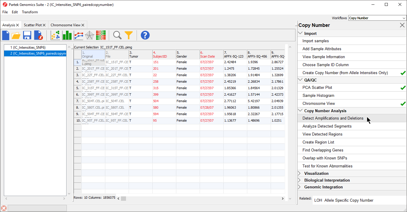
Figure 1. Invoking Detect Amplifications and Deletions
The Detect Amplifications and Deletions dialog will give you the option to choose Genomic Segmentation or HMM Region Detection (Figure 2).
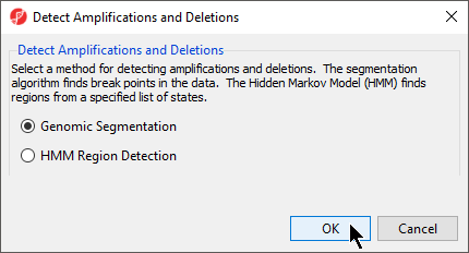
Figure 2. Select a method for detecting amplifications and deletions
- Select Genomic Segmentation
- Select OK
The Genomic Copy Number Segmentation dialog gives options for setting segmentation parameters and the configuring the region report (Figure 3).
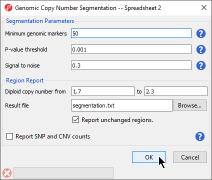
Figure 3. Configuring the Genomic Copy Number Segmentation dialog
- Set Minimum genomic markers to 50
- Leave the rest of the parameters set to default values as shown (Figure 3)
- Select OK
The Genomic Segmentation task is divided into two steps. In the first step, each region is compared to an adjacent region to determine whether both have the same average copy number and whether a breakpoint can be inserted. This is determined by first using a two-sided t-test to compare the average intensities of adjacent regions and then checking whether the corresponding cut-off p-value is below the specified P-value threshold. The genomic size of a region is defined by the number of genomic markers in the region, Minimum genomic markers, while the magnitude of the significant difference between two regions is controlled by Signal to noise, which can be thought of as the difference in copy numbers between the regions. If the t-test is significant, the copy number of the region differs significantly from its nearest neighbors. However, a second step is needed to detemine whether the difference is due to amplificaiton or deletion. In this second step, two one-sided t-tests are used to compare the mean copy number in the region with the expected diploid copy number. For a detailed explanation of the genomic segmenetation procedure, please consult our Genomic Segmentation white paper. For more detailed information about fine-tuning the parameters of your copy number analysis, please consult our guide, Optimizing Copy Number Segmentation.
The resulting spreadsheet, segmentation, shows one row per genomic region per sample (Figure 4). The columns provide the following information:
1-4: Genomic location of the region
5. Sample ID
6. Description of the copy number change
7. The length of the region (in base pairs)
8. The number of markers in the region
9. Markers density in the region (region length in base pairs divided by the number of markers)
10. Geometric mean of the copy number of all the markers in the region
11. Minimum p-value of the one-sided t-tests of the difference of the copy number in column 10 vs. the diploid range
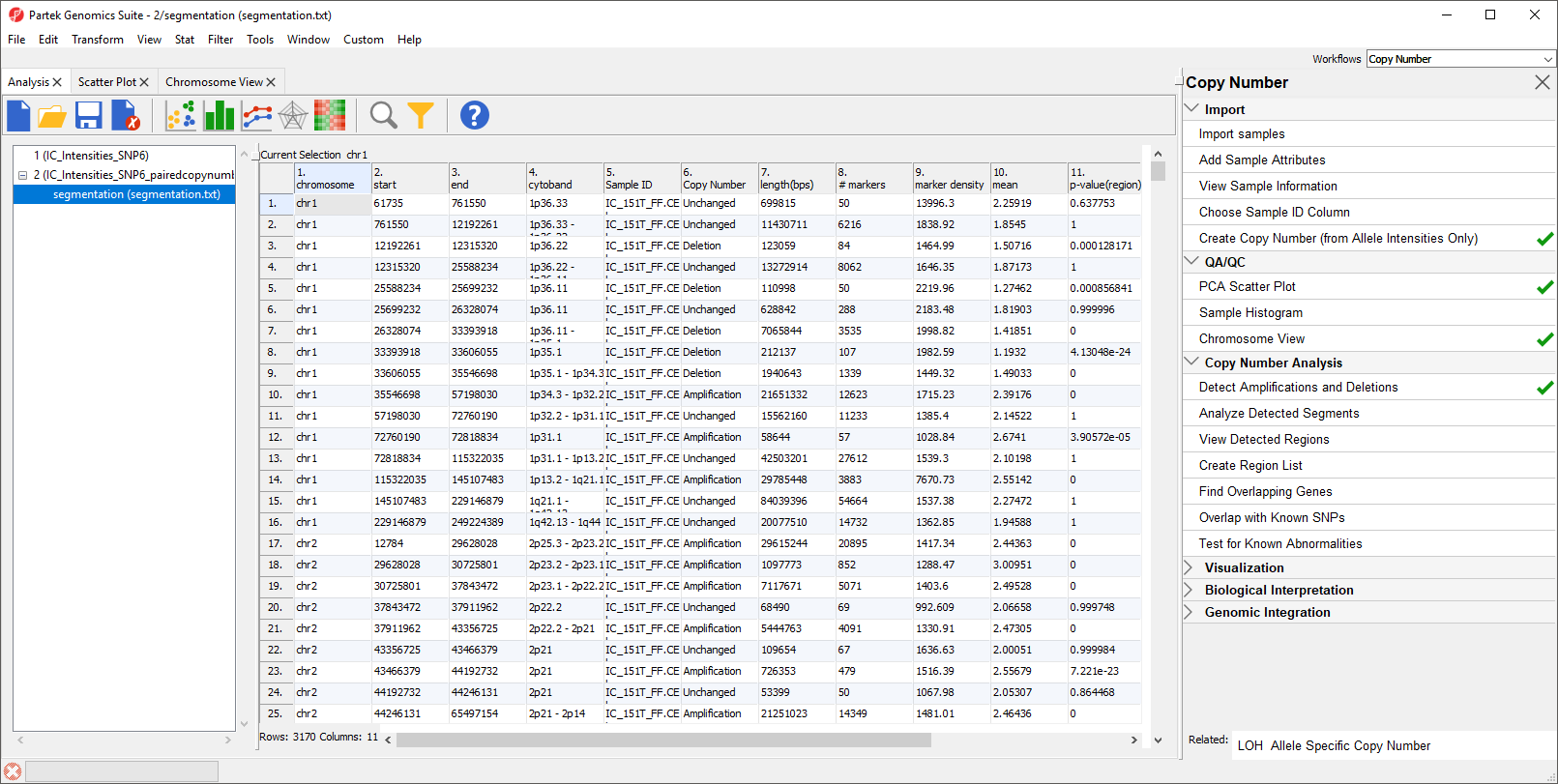
Figure 4. Viewing the segmentation spreadsheet
If desired, you can use Merge Adjacent Regions under Tools in the main toolbar to combine similar regions.
Visualizing regions of interest
Individual regions of interest can be visualized using Chromosome View.
- Right-click a row header in the segmentation spreadsheet
- Select Browse to location from the pop-up menu
Alternatively, you can visualize results at the whole chromosome level.
- Select the segementation spreadsheet
- Select Chromosome View from the QA/QC section of the workflow
The Genomic Segementation track displays the segmentation results (Figure 5). Each line in the track represents a sample. Amplified, deleted, and unchanged regions are shown in red, blue, and white, respectively. The Profile track now also includes information from the segmentation spreadsheet for the selected sample.
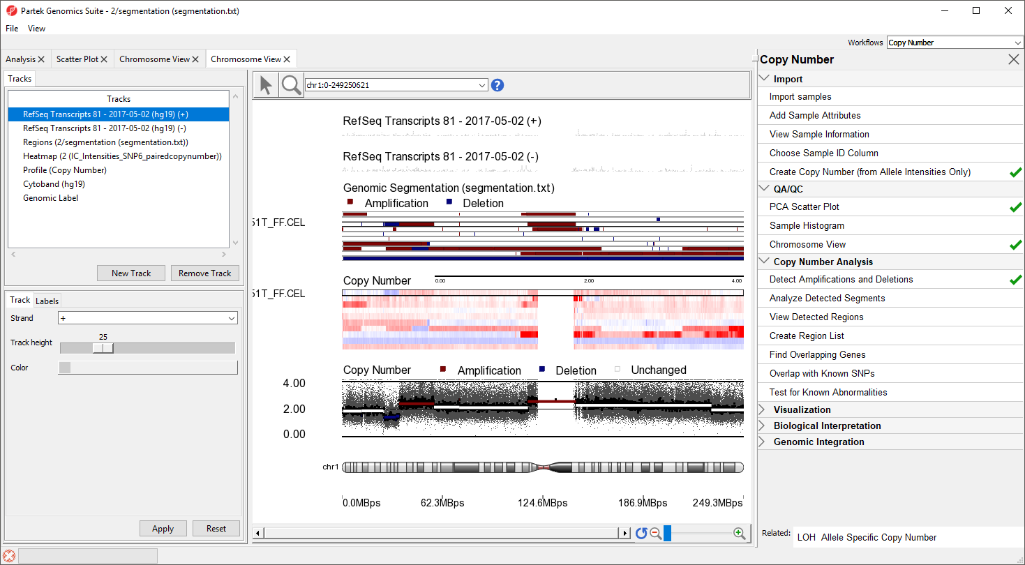
Figure 5. Segmentation results shown as regions of amplification and deletion in each sample
Analyzing shared regions of copy number variation
Amplified and deleted regions in each sample have been detected, we can compare the regions across multiple samples to detect copy number changes that are shared by multiple samples.
- Select Analyze detected segments from the Copy Number Analysis section of the workflow
The Analyze Segments task (Figure 6) can test for associations between copy number variations and sample categories using the χ2 test. In this tutorial, all pairs share the sample phenotype, so we will not test for associations.
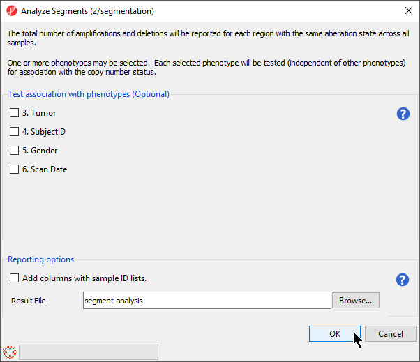 Figure 6. Viewing the Analyze segments dialog
- Leave all boxes unchecked
- Select OK to run the Analyze Segements task
The task generates a new spreadsheet, summary (segment-analysis) (Figure 7), with one region per row. The columns provide the following information:
1-4. Genomic locations of the regions
5. Total number of samples
6-7. Number of samples with amplifications and the average amplified copy number, respectively
8-9. Number of samples with deletions and the average deleted copy number, respectively
10. Total number of samples with copy number abberations
11-12. Number of samples with no change in copy number and the average copy number in those samples, respectively
13. Number of markers in the region
14. Length of the region (in base pairs)
15+. Two columns per sample - the average copy number in each sample as well as the copy number change status of the sample sample (e.g., amplified, deleted, unchanged, depending on the copy number and the threshold for unchanged defined in the Genomic Segementation dialog)
A "?" indicates that a region with the particular characterisitic does not exist or cannot be computed. For example, if a region is not amplified in any of the samples, the average amplified copy number will be shows as "?". This list may be filtered to contain only regions that meet user-specified criteria as discussed in the next section of the tutorial.
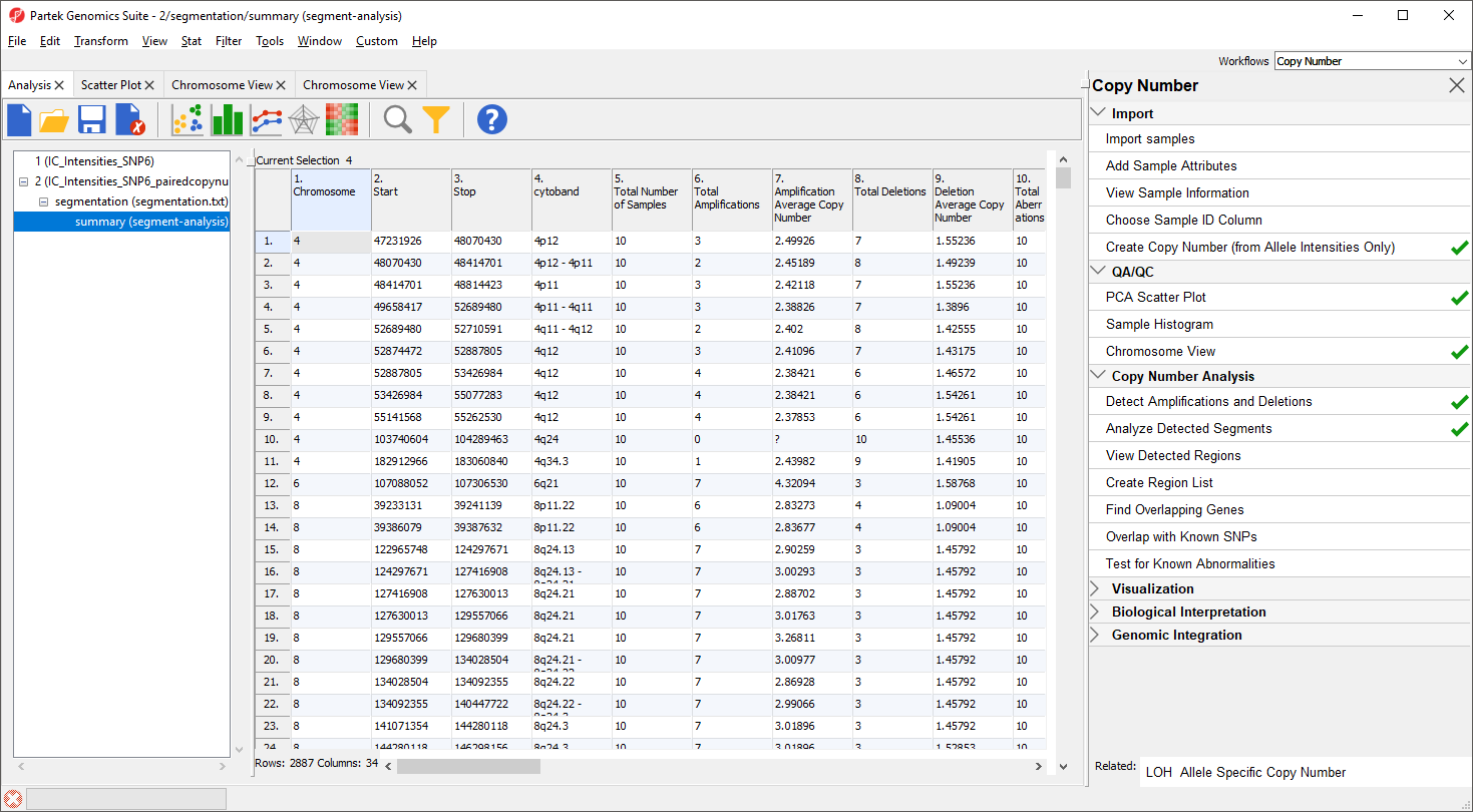
Figure 7. Viewing the results of Analyze Detected Segments
Visualizing shared regions of copy number variation
To get an overiew of the common abberations in the group of samples over the entire genome we can use View Detected Regions.
- Select View Detected Regions
The View Detected Regions dialog (Figure 7) allows you to select the spreadsheet with genomic regions and choose between histogram and copy number classification plots.
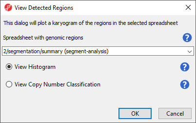
Figure 8. View Detected Regions dialog
- Select summary (segment-analysis) from the drop-down menu
- Select View Histogram
- Select OK
The plot will open in a new tab titled Karyogram View (Figure 8).
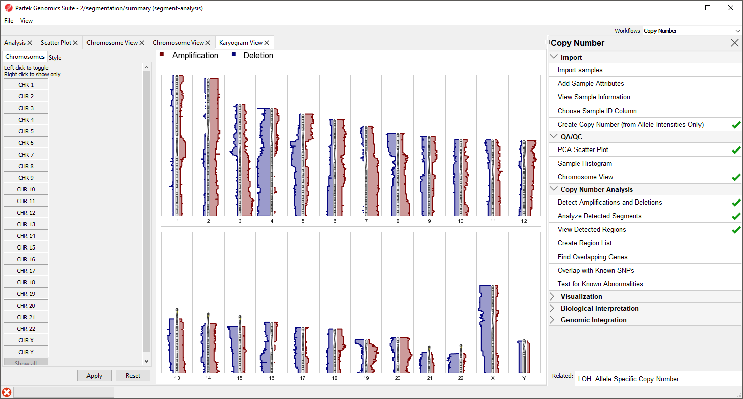
Figure 9. Viewing amplification and deletion histograms using Karyogram View
The Karyogram View shows each chromosome with red and blue histograms on either side corresponding to amplification and deletion, repsectively. The histogram height reflects the number of samples that share either amplification of deletion a that particular region. For example, the long arms of chromosomes 3 and 7 are amplified in the majority of samples and most samples share a deletion in the long arm of chromosome 4.
Mousing over the chromosome will give cytoband information, mousing over the histogram will give the number of shared regions at each position and the number of samples sharing the type of variation. Both the menu and display may be used to control which chromosomes are displayed; left-click in the menu to toggle a chromosome on/off and right click in the menu or graph to show only that chromosome.
Alternatively, we can use the Copy Number Classification plot to get a more sample-centric view.
- Select View Detected Regions
- Select View Copy Number Classification
- Select OK
The Copy Number Classificaiton also utilizes Karyogram View to provides an overview of all the samples and the copy number of regions on each chromosome (Figure 9).
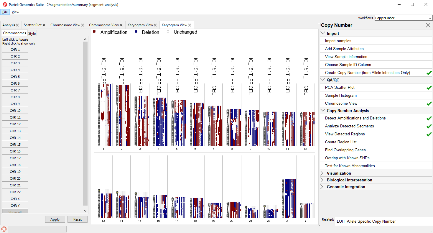
Figure 10. Viewing the Copy Number Classification plot
Each sample is drawn as a separate column next to the chromosome. Amplified regions are depicted in red, deleted regions in blue, and regions with no copy number change in white. Sample names are given accross the top of each column. For greater detail, try viewing fewer chromosomes.
Additional Assistance
If you need additional assistance, please visit our support page to submit a help ticket or find phone numbers for regional support.


| Your Rating: |
|
Results: |

|
34 | rates |
Overview
Content Tools