Cytoband Track

By default, the Chromosome view shows a cytoband track at the top of the canvas. If a cytoband file for your genome has not been added to Partek^® Flow^®, a warning will appear (Figure 1). In that case, go to the Library File Management page and download or create a cytoband file.

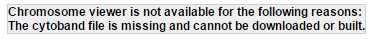
Figure 1. Warning message indicating that Chromosome view can not be launched because of missing cytoband file

The red box (Figure 2) indicates the part of the chromosome that is currently depicted on the canvas.

The sequence of the reference genome is added to the Chromosome view by default, as long as it has been added to the respective genome on the Library File Management page. However, its presence (or absence) in the viewer depends on the current magnification. At low power, the track is hidden and you will see the message - Track hidden (zoom to view). At high power, on the other hand, the Reference genome track becomes visible (Figure 3) and is supplemented by the genomic coordinates (below the sequence). A vertical guide helps you to align the bases between Aligned reads and Reference genome tracks. Depending on the reference genome file, some bases may be shown in lowercase letters, symbolizing repetitive sequences, or other sequences masked by a tool such as RepeatMasker.

If a variant database file (such as dbSNP) for your genome is present on the Library File Management page, you will be able to include variant annotation track in your visualization (to add a variant database to the viewer, use the control panel on the right).

The variants will be shown adjacent to the Reference genome track (Figure 3). If the database contains no frequency information on alternative alleles, the alleles will be drawn as bars (an example is the SNP on the left in Figure 4). If the frequency information is available, the relative frequency of each variant will be represented by a column (the SNP on the right in Figure 4).

Figure 4. Reference genome track with added variant annotation: single nucleotide variants present in the chosen database are depicted as bars (if no frequency information is available) or columns (columns reflect relative frequency of each alternative allele as stored in the database)

Note that the frequency information for each allele will be parsed out from the chosen database. That information can be retrieved by selecting a variant using the selection mode and will be shown in the Selection details section of the control panel. Using the example shown in Figure 4, the details of the left database variant can be seen in Figure 5. The most frequent allele at that locus is G (hence, the yellow column is plotted above the Reference genome track), which matches the base call of the reference genome.

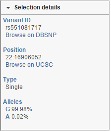
Figure 5. Selection details section of the control panel showing details of a SNV, as present in the selected database

If your variant database stores indels, they will be depicted using green (insertion) or red (deletion) symbols (Figure 6) pointing to deleted bases.

Figure 6. Reference genome track with added variant annotation: insertions are shown in green, deletions in red. In this example, an insertion of a single base has described in the database, between G and T. An adjacent deletion of T and C bases has also been seen before

Other Annotation Tracks

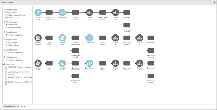
Additional annotation tracks can be added to the viewer with the help of the Select tracks dialog as long as they have been associated with the genome you are working on in the Library File Management.

A common choice of an additional track is a transcript database, such as RefSeq (Figure 7). All the database entries are displayed, using a common depiction of exons as boxes and introns as lines connecting them. Untranslated regions (UTRs) are seen as narrow boxes. The arrows indicate directionality.

Figure 7. Transcript database track: a gene with two transcripts is shown as an example. Exons are plotted as boxes and introns as lines connecting them. Untranslated regions (UTRs) are seen as narrow boxes. The arrows indicate directionality

Your Rating:

Thanks for voting!

Please Wait

Results:

30

rates