In RNA-seq data analysis, after alignment, the most common step is to estimate gene or/and transcript expression abundance, the expression level is represented by read counts. There are three options in this step:
- Quantify to annotation model (Partek E/M)
- Quantify to transcriptome (Cufflinks)
- Quantify to reference (Partek E/M)
The three options will be discussed below.
Quantify to annotation model (Partek E/M)
When the reads are aligned to a genome reference, e.g. hg38, the quantification is performed on transcriptome, you need to provide the annotation model file of the transcriptome.
Quantification dialog
If the alignment was generated in Partek® Flow®, the genome assembly will be displayed as text on the top of the page (Figure 1), you do not have the option to change the reference.
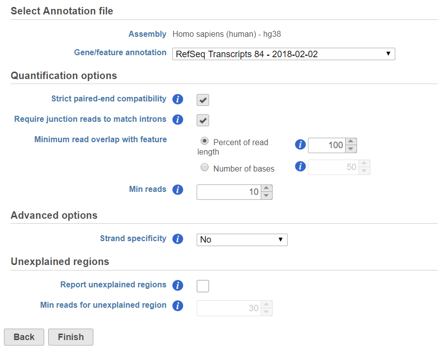 Figure 1. Quantify to annotation model(Partek E/M) dialog
If the bam file is imported, you need to select the assembly with which the reads were aligned to, and which annotation model file you will use to quantify from the drop-down menus (Figure 2).
Figure 2. Specify the genome assembly with which the bam files are generated from and transcriptome annotation from the drop-down menu
In the Quantification options section, when the Strict paired-end compatibility check button is selected, paired end reads will be considered compatible with a transcript only if both ends are compatible with the transcript. If it is not selected, reads with only one end have alignment that is compatible with the transcript will also be counted for the transcript .
If the Require junction reads to match introns check button is selected, only junction reads that overlap with exonic regions and match the skipped bases of an intron in the transcript will be included in the calculation. Otherwise, as long as the reads overlap within the exonic region, they will be counted. Detailed information about read compatibility can be found in the Understanding Reads tutorial.
There are five options in Strand specificity drop-down selection. We recommend verifying with the data source how the NGS library was prepared to ensure correct option selection.
Some library preparations reverse transcribe the mRNA into double stranded cDNA, thus losing strand information. In this case, the total transcript count will include all the reads that map to a transcript location. Others will preserve the strand information of the original transcript by only synthesizing the first strand cDNA. Thus, only the reads that have sense compatibility with the transcripts will be included in the calculation.
In the options, forward means the strand of the read must be the same as the strand of the transcript while reverse means the read must be the complementary strand to the transcript (Figure 3). The dash separates first- and second-in-pair. For paired end reads, we determine these by the flag information of the read in the BAM file. For single end reads, they are treated as the first read of paired end read. Briefly, the Strand specificity options are:
- No: Reads will be included in the calculation as long as they map to exonic regions, regardless of the direction.
- Auto-detect: The first 200,000 reads will be used to examine the strand compatibility with the transcripts. Two percentages are calculated: (1) the percentage of reads whose first-in-pair is the same strand as the transcript and second-in-pair is the opposite strand to transcript, (2) the percentage of reads whose first-in-pair is the opposite strand to transcript and second-in-pair is the same strand as the transcript. If the 1st percentage is higher than 75%, the Forward-Reverse option will be used. If the 2nd percentage is higher than 75%, the Reverse-Forward option will be used. If neither of the percentages exceed 75%, No option will be used.
- Forward – Reverse: this option is equivalent to the --fr-secondstrand option in Cufflinks [1]. First-in-pair is the same strand as the transcript, second-in-pair is the opposite strand to the transcript.
- Reserve – Forward: this option is equivalent to --fr-firststrand option in Cufflinks. First-in-pair is the opposite strand to the transcript, second-in-pair is the same strand as the transcript. The Illumina TruSeq Stranded library prep kit is an example of this configuration.
- Forward – Forward: Both ends of the read are matching the strand of the transcript. Generally colorspace data generated from SOLiD technology would follow this format
Figure 3. Illustration of the three types of strand specific assays on paired end reads. _R1 and _R2 means read first-in pair and second-in-pair respectively. Arrows indicate strand directions.
Minimum read overlap with feature can be specified in percentage of read length or number of bases. By default, a read has to be 100% within a feature. You can allow some overhanging bases outside the exonic region by modifying these parameters.
If the Report unexplained regions check button is selected, an additional report will be generated on the reads that are considered not compatible with any transcripts in the annotation provided. Based on the Min reads for unexplained region cutoff, the adjacent regions that meet the criteria are combined and region start and stop information will be reported.
In the annotation file, there might be multiple features in the same location, or one read might have multiple alignments, so the read count of a feature might not be an integer. Our white paper on the Partek E/M algorithm has more details on Partek’s implementation the E/M algorithm initially described by Xing et al. [2]
Quantify to annotation model (Partek E/M) output
Depending on the annotation file, the output could be one or two data nodes. If the annotation file only contains one level of information, e.g. miRNA annotation file, you will only get one output data node. On the other hand, if the annotation file contains gene level and transcript level information, such as those from the Ensembl database, both gene and transcript level data nodes will be generated. If two nodes are generated, the Task report will also contain two tabs, reporting quantification results from each node. Each report has two tables. The first one is a summary table displaying the coverage information for each sample quantified against the specified transcriptome annotation (Figure 4).
Figure 4. Summary of raw reads mapping to genes based on the RefSeq annotation file provided. Note that the Gene-level tab is selected.
The second table contains feature distribution information on each sample and across all the samples, number of features in the annotation model is displayed on the table title (Figure 5).
Figure 5. Summary of feature distribution statistics
The bar chart displaying the distribution of raw read counts is helpful in assessing the expression level distribution within each sample. The X-axis is the read count range, Y axis is the number of features within the range, each bar is a sample. Hovering your mouse over the bar displays the following information (Figure 6):
- Sample name
- Range of read counts, “[ “represent inclusive, “)” represent exclusive, e.g. [0,0] means 0 read counts; (0,10] means the range is greater than 0 count but less than and equal to 10 counts.
- Number of features within the read count range
- Percentage of the features within the read count range
Figure 6. Bar chart on distribution of raw read counts in each sample
The coverage breakdown bar chart is a graphical representation of the reads summary table for each sample (Figure 7)
Figure 7. Coverage breakdown bar chart, it is a graphical presentation of summary table on raw reads mapping to transcription based on the annotation file provided
In the box-whisker plot, each box is a sample on X-axis, the box represents 25th and 75th percentile, the whiskers represent 10th and 90th percentile, Y-axis represents the read counts, when you hover over each box, detailed sample information is displayed (Figure 8).
Figure 8. Box-whisker plot on read count distribution in each sample, when mouse over a box, detailed information on the box is displayed.
In sample histogram, each line represents a sample and the range of read counts are divided into 20 bins. Clicking on a sample in the legend will hide the line for that specific sample. Hovering over each circle displays detailed information about the sample and that specific bin (Figure 9). The information includes:
- Sample name
- Range of read counts, “[ “represent inclusive, “)” represent exclusive
- Number of features within the read count range in the sample
Figure 9. Sample histogram plot, when mouse over each circle, detailed information is displayed
The box whisker and sample histogram plots are helpful for understanding the expression level distribution across samples. This may indicate that normalization between samples might be needed prior to downstream analysis.
Quantify to transcriptome (Cufflinks)
Cufflinks assembles transcripts and estimates transcript abundances on aligned reads. Implementation details are explained in Trapnell et al. [1]
The Cufflinks task has three options that can be configured (Figure 10):
Figure 10. Cufflinks configuration dialog
- Novel transcript : this option does not require any annotation reference, it will do de novo assembly to reconstruct transcripts and estimate their abundance
- Annotation transcript : this option requires an annotation model to quantify the aligned reads to known transcripts based on the annotation file.
- Novel transcript with annotation as guide: this option requires an annotation file to quantify the aligned reads to known transcripts as well as assemble aligned reads to novel transcripts. The results include all transcripts in the annotation file plus any novel transcripts that are assembled.
When the Use bias correction check box is selected, it will use the genome sequence information to look for overrepresented sequences and improve the accuracy of transcript abundance estimates.
Quantify to reference (Partek E/M)
This task does not need an annotation model file, since the annotation is retrieved from the BAM file itself. The sequence names in the BAM files constitute the features with which the reads are quantified against
This task is generally performed on reads aligned to a transcriptome, e.g when a species does not have a genome reference, and the bam files contain transcriptome information. In this case, the features for this quantification task are the reference sequence names in the input bam files.
There are two parameters in Quantify to reference (Figure 11):
Figure 11. Quantify to reference dialog
- Min coverage: will filter out any features (sequence names) that have fewer reads across all samples than the value specified
- Strict paired-end compatibility: this only affects paired end data. When it is checked, only reads that have two ends aligned to the same feature will be counted. Otherwise, reads will still be counted as exonic compatible reads even if the mate is not compatible with the feature
The output data node will display a similar Task report as the Quantify to annotation model task.
References
- Trapnell C, Williams B, Pertea G, et al. Transcript assembly and quantification by RNA-Seq reveals unannotated transcripts and isoform switching during cell differentiation. Nature Biotech. 2010; 28:511-515.
- Xing Y, Yu T, Wu YN, Roy M, Kim J, Lee C. An expectation-maximization algorithm for probabilistic reconstructions of full-length isoforms from splice graphs. Nucleic Acids Res. 2006; 34(10):3150-60.
Additional Assistance
If you need additional assistance, please visit our support page to submit a help ticket or find phone numbers for regional support.


| Your Rating: |
|
Results: |

|
3 | rates |
Overview
Content Tools