Binding sites for the DNA-binding protein of interest are indicated by enriched sequencing read density. Because each single-end read only covers one end of an immunoprecipitated DNA fragment, enriched regions will have two adjacent peaks of increased sequencing read density from reads on the forward and reverse strands. To merge these peaks, each read is extended in the 3' direction by the effective fragment length, converting reads into estimated fragments. Overlapping estimated fragments are then merged into peaks. For peak detection, the genome is divided into bins of a user-defined size and the number of estimated fragments that fall in each bin is calculated. A zero-truncated negative binomial model, appropriate for data is fitted to the bin counts and all regions that are enriched above a user-defined false discovery rate (FDR) are called as peaks.
Using the effective fragment length calculated by Cross Strand-Correlation, each read is extended in the 3' direction by the effective fragment length and overlapping extended reads are merged into a single peak. For paired-end reads, the distance between paired reads is used as the fragment length and overlapping fragments are merged into peaks. For peak detection, Partek Genomics Suite divides the genome into windows of a user-defined size and counts the number of fragments whose mid-points fall within each window. A statistical test is then applied to determine which peaks are significant. See the ChIP-Seq white paper for more information on the peak-finding algorithm and tips for setting the Fragment extension and window sizes.
- Select spreadsheet 1 (ChIP-Seq) from the spreadsheet tree
- Select Detect peaks from the Peak Analysis section of the ChIP-Seq workflow
The Peak Detection dialog will open. We will configure the dialog as shown (Figure 1).
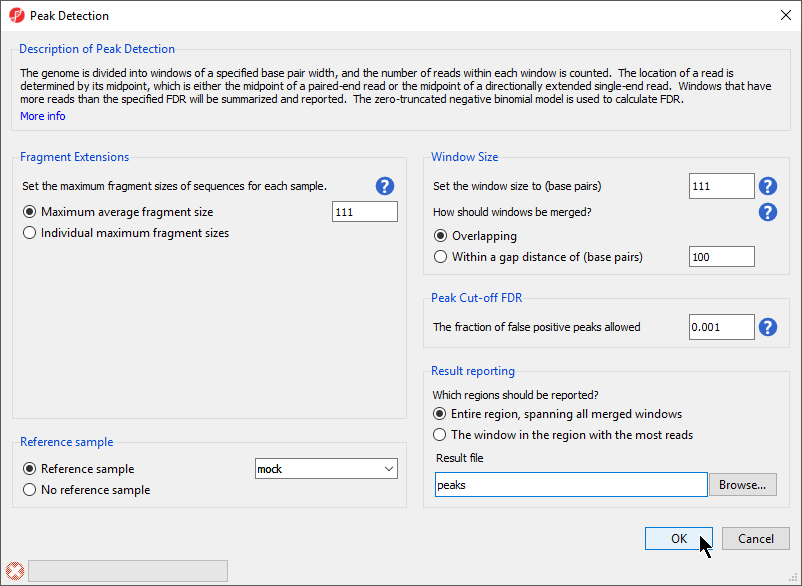
Figure 1. Configuring the peak detection dialog. The appropriate settings for will depend on your experimental design and data.
- Select Maximum average fragment size for Fragment Extensions
- Set Maximum average fragment size to 111
Maximum average fragment size is based on your experimental design: the size of the fragment pulled-down by immunoprecipitation, the fragment sizes produced by DNA fragmentation, the fragment length selected by size exclusion, or the effective fragment length calculated by Cross Strand-Correlation. If you have used an antibody that binds DNA as the control antibody such as an IgG control, you could use different fragment lengths for each sample based on its effective fragment length by selecting the Individual maximum fragment sizes option. Here, we have chosen the effective fragment length of 111 base pairs calculated using Cross Strand-Correlation.
- Select Reference sample from Reference sample
- Select mock from the Reference sample drop-down menu
- Set Set the window size to (base pairs) to 111
The peak detection algorithm divides the genome into windows to find windows with enriched for reads based on FDR value. Here, we have chosen to match the window and individual maximum fragment sizes.
- Select Overlapping for How should windows be merged?
- Set The fraction of false positive peaks allowed to 0.001
The Peak Cut-off FDR determines the cut-off for calling peaks. Setting a lower value demands greater differences between mock and chip samples fora peak to be called; a false discovery rate of 0.001 anticipates 1 false positive per 1000 peaks called.
- Select Entire region, spanning all merged windows for Which regions should be reported?
Optimal peak detection settings are dependent on your experimental design and data so fine tuning may be required. Because transcription factor binding sites tend to have localized and sharp clusters of reads, the window size used during the analysis of a transcription factor study can be left relatively small, approximately the same as the average fragment length, and the option to allow for gaps between enriched windows does not need to used. Additionally, Region in the window with most reads could be selected to report a more narrow region for each peak call. Conversely, histone modification peaks tend to be subtle and diffuse. To analyze histone modification ChIP-seq data, larger window sizes, combining neighboring windows into larger windows using Within a gap distance of, and reporting entire regions using Entire region, spanning all merged windows might be appropriate.
A convenient way to visualize the relationship between window size and gap size is to select the More info link at the top of the Peak Detection dialog box. A simulated read count histogram will open below the Description of Peak Detection section (Figure 2). The blue bars underneath the histogram will reflect how regions are detected and reported using your current Peak Detection settings. Try changing the How should windows be merged or Which regions should be reported? options to visualize their effects on peak detection.
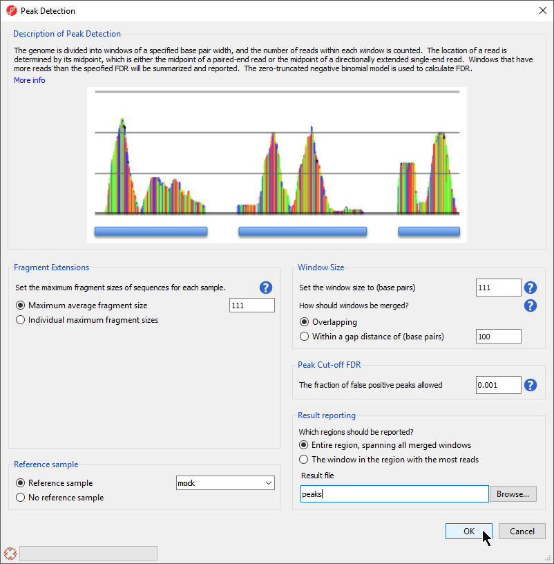 Figure 2. The visual guide helps show the impact of window size and result reporting settings on peak calling.
- Select OK to run the peak detection algorithm with your chosen settings
Peak Detection generates a new child spreadsheet, regions (peaks) (Figure 3).

Figure 3. Peaks spreadsheet lists regions with significant peak enrichment with one row per region.
A few of the columns contents merit clarification.
Additional Assistance
If you need additional assistance, please visit our support page to submit a help ticket or find phone numbers for regional support.


| Your Rating: |
|
Results: |

|
1 | rates |
Overview
Content Tools