Join us for an event September 26!
How to Streamline RNA-Seq analysis and increase productivity—point, click, and done
Each row of the spreadsheet (Figure 1) corresponds to a single sample. The first column is the names of the .idat files and the remaining columns are the array probes. The table values are β-values, which correspond to the percentage methylation at each site. A β-value is calculated as the ratio of methylated probe intensity over the overall intensity at each site (the overall intensity is the sum of methylated and unmethylated probe intensities).
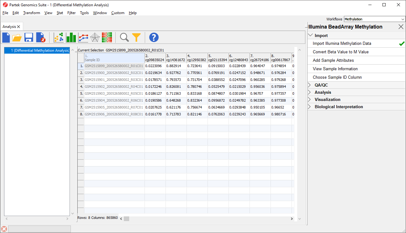
Figure 1. Spreadsheet after .idat file import: samples on rows (Sample IDs are based on file names), probes on columns, cell values are functionally normalized beta values (default settings)
An alternative metric for measurement of methlyation levels are M-values. β-values can be easily converted to M-values using the following equation:
M-value = log2( β / (1 - β))
An M-value close to 0 for a CpG site indicates a similar intensity between the methylated and unmethylated probes, which means the CpG site is about half-methylated. Positive M-values mean that more molecules are methylated than unmethylated, while negative M-values mean that more molecules are unmethylated than methylated. As discussed by Du and colleagues, the β-value has a more intuitive biological interpretation, but the M-value is more statistically valid for the differential analysis of methylation levels.
Because we are performing differential methylation analysis, we need to convert our data to from β-values to M-values.
- Select Convert Beta Value to M Value from the Import section of the Illumina BeadArray Methylation workflow
The original data (β-values) will be overwritten.
- Select (
 ) from the icon bar to save the current spreadsheet
Before we can perform any analysis, the study samples need to be organized into their experimental groups.
- Select Add Sample Attributes from the Import section of the Illumina BeadArray Methylation workflow
- Select Add a Categorical Attribute from the Add Sample Attributes dialog (Figure 2)
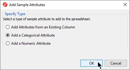
Figure 2. Adding sample attributes. Adding Attributes from an Existing Column can be used to split file names into sections, based on delimiters (e.g. _, -, space etc.). Adding a Numeric or Categorical Attribute enables the user to manually specify sample attributes
- Select OK
The Create categorical attribute dialog (Figure 3) allows us to create groups for a categorical attribute. By default, two groups are created, but additional groups can be added.
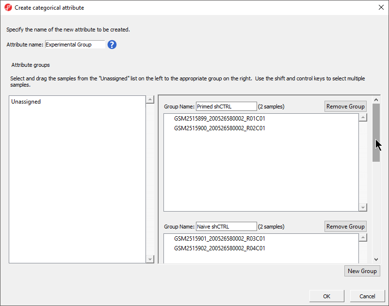
Figure 3. Create Categorical Attribute is used to define new groups and assign samples to them. The name of new column (attribute) is specified in the Attribute name field, group labels (attribute levels) are specified in the Group Name fields. To assign samples to groups, use drag and drop (to select more than one, use Ctrl or Shift buttons)
- Select New Group twice to add two additional groups
- Set Attribute name: to hPSC
- Rename the four groups Primed, Naive, shPOU5F1, and shNANOG
- Drag and drop the samples from the Unassigned list to their groups as listed in the table below
| Sample ID | Group Name |
|---|---|
GSM2515899_200526580002_R01C01 | Primed |
GSM2515900_200526580002_R02C01 | Primed |
GSM2515901_200526580002_R03C01 | Naive |
GSM2515902_200526580002_R04C01 | Naive |
GSM2515903_200526580002_R05C01 | shPOU5F1 |
GSM2515904_200526580002_R06C01 | shPOU5F1 |
GSM2515905_200526580002_R07C01 | shNANOG |
GSM2515906_200526580002_R08C01 | shNANOG |
There should now be four groups with two samples in each group (Figure 4).
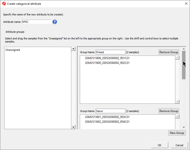
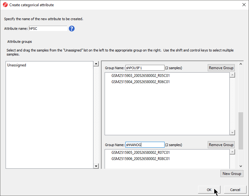
Figure 4. hPSC attribute with four groups - Primed, Naive, shPOU5F1, and shNANOG - of two samples per group
- Select OK
- Select No from the Add another categorical attribute dialog
- Select Yes to save the spreadsheet
A new column as been added to spreadsheet 1 (Differential Methylation Analysis) with the experimental group of each sample (Figure 5).
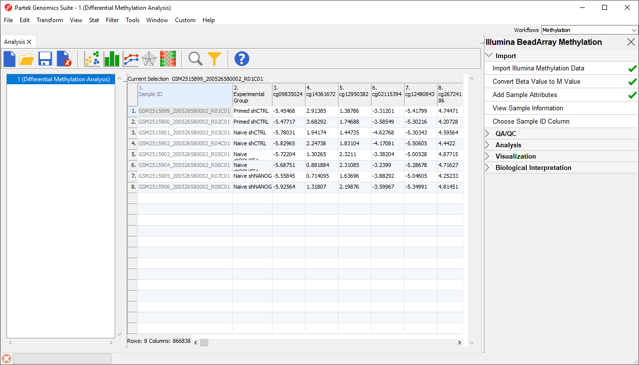
Figure 5. Added experimental group as a sample attribute
Additional Assistance
If you need additional assistance, please visit our support page to submit a help ticket or find phone numbers for regional support.


| Your Rating: |
|
Results: |

|
0 | rates |
Overview
Content Tools