Once the .idat files are imported, you will be facing the Scatter Plot. To move forward with the tutorial, switch to the Analysis tab and take a look at the top level (i.e. initial) spreadsheet (Figure 1). Samples identifiers are the names of the .idat files as shown by the Sample ID column while all the remaining columns are the array probes.
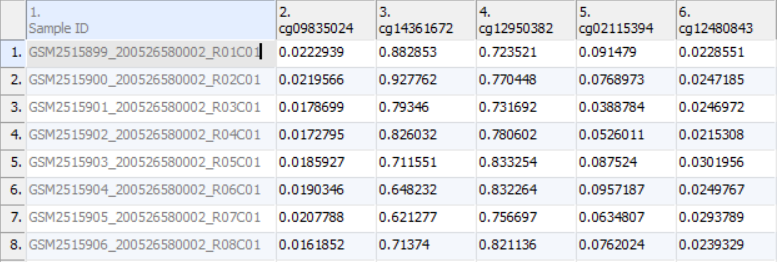 Figure 1. Spreadsheet after .idat file import: samples on rows (Sample IDs are based on file names), probes on columns, cell values are functionally normalized beta values (default settings)
As discussed in the previous chapter, the values in the cells are normalized β-values, which correspond to the percentage of methylation at each site and are calculated as the ratio of methylated probe intensity over the overall intensity at each site (the overall intensity is the sum of methylated and unmethylated probe intensities). An alternative metric for measurement of methlyation levels are M-values. β-values can be easily converted to M-values using the following equation:
M-value = log2( β / (1 - β))
Here's the interpretation: a M-value close to 0 indicates a similar intensity between the methylated and unmethylated probes, which means the CpG site is about half-methylated. Positive M-values mean that more molecules are methylated than unmethylated, while negative M-values mean that more molecules are unmethylated than methylated. As discussed by Du and colleagues, the β-value has a more intuitive biological interpretation, but the M-value is more statistically valid for the differential analysis of methylation levels.
Therefore, the differential methylation analysis of the tutorial data will be performed on the M-values; select Convert Beta Value to M Value from the workflow. Note that the original data (β-values) will be overwritten.
Before proceeding to exploratory data analysis, the study samples need to be organized in four groups, two biological replicates each. In the Import section of the workflow, select Add Sample Attributes and, in the next dialog (Figure 2), Add a Categorical Attribute (and then OK).
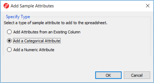 Figure 2. Adding sample attributes. Adding Attributes from an Existing Column can be used to split file names into sections, based on delimiters (e.g. _, -, space etc.). Adding a Numeric or Categorical Attribute enables the user to manually specify sample attributes
The following dialog is Create Categorical Attribute (Figure 3). The Attribute name filed specifies the name of the new column (attribute), while the groups (levels of the attribute) are specified in the Group Name fields. By default, two groups are created, but additional ones can be added using the New Group button. Finally, drag and drop the samples from the Unassigned list to their matching groups.
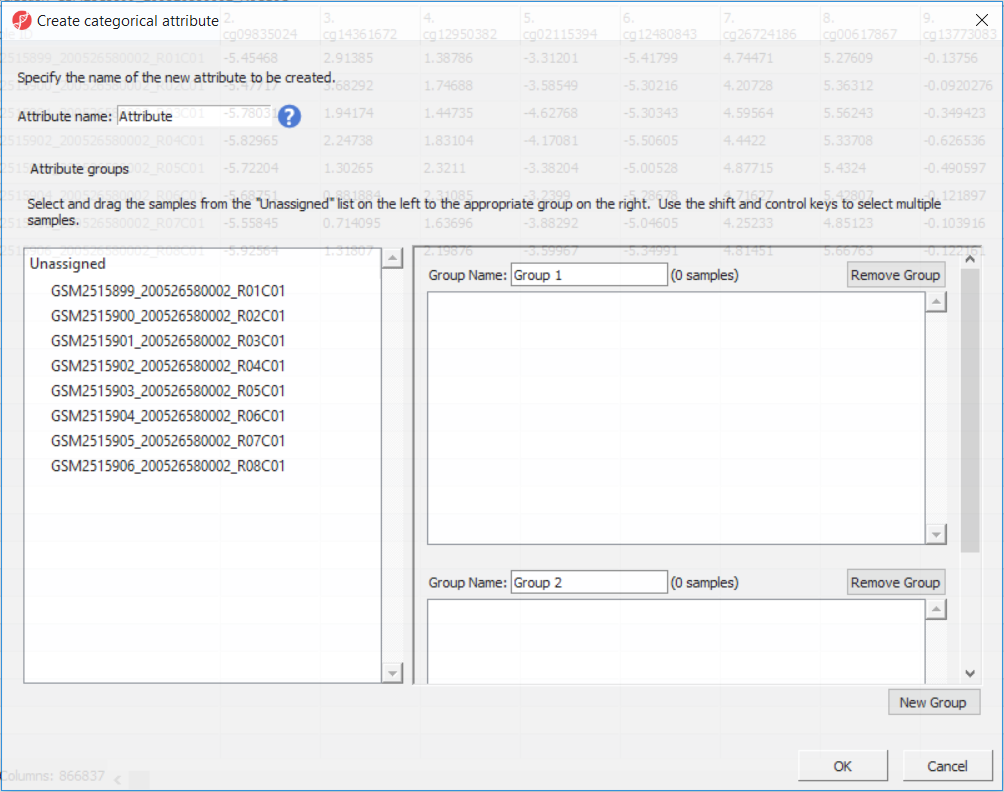 Figure 3. Create Categorical Attribute is used to define new groups and assign samples to them. The name of new column (attribute) is specified in the Attribute name field, group labels (attribute levels) are specified in the Group Name fields. To assign samples to groups, use drag and drop (to select more than one, use Ctrl or Shift buttons)
Section Heading
Section headings should use level 2 heading, while the content of the section should use paragraph (which is the default). You can choose the style in the first dropdown in toolbar.
Additional Assistance
If you need additional assistance, please visit our support page to submit a help ticket or find phone numbers for regional support.


| Your Rating: |
|
Results: |

|
1 | rates |
Overview
Content Tools