Page History
...
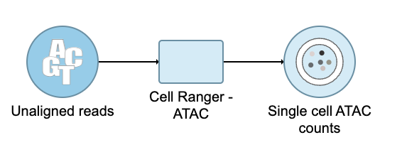
This guide illustrates how to process FASTQ files produced using the 10x Genomics Chromium Single Cell ATAC assay to obtain a Single cell counts data node, which is the starting point for analysis of single-cell ATAC experiments.
If you are new to Partek® Flow®Partek Flow, please see Getting Started with Your Partek Flow Hosted Trial for information about data transfer and import and Creating and Analyzing a Project for information about the Partek Flow user interface.
...
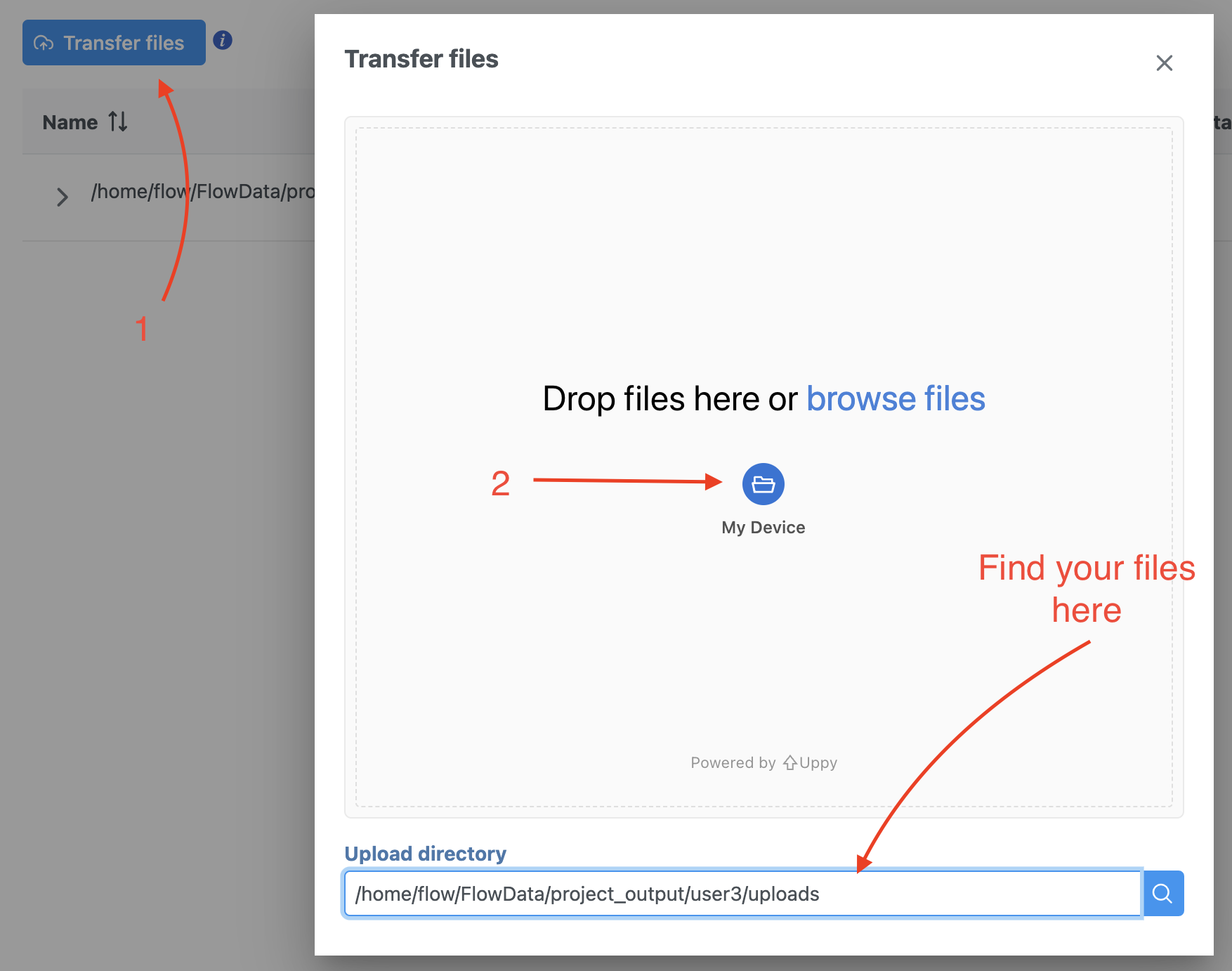
We recommend uploading your FASTQ files (fastq.gz) to a folder on your Partek® Flow® Partek Flow server before importing them into a project. Data files can be transferred into Flow from the Home page by clicking the Transfer file button (Figure 1). Following the instruction In Figure 1 to complete the data transfer. Users have the option to change the Upload directory by clicking the Browse button and either select another existing directory or create a new directory.
...
| Numbered figure captions | ||||
|---|---|---|---|---|
| ||||
|
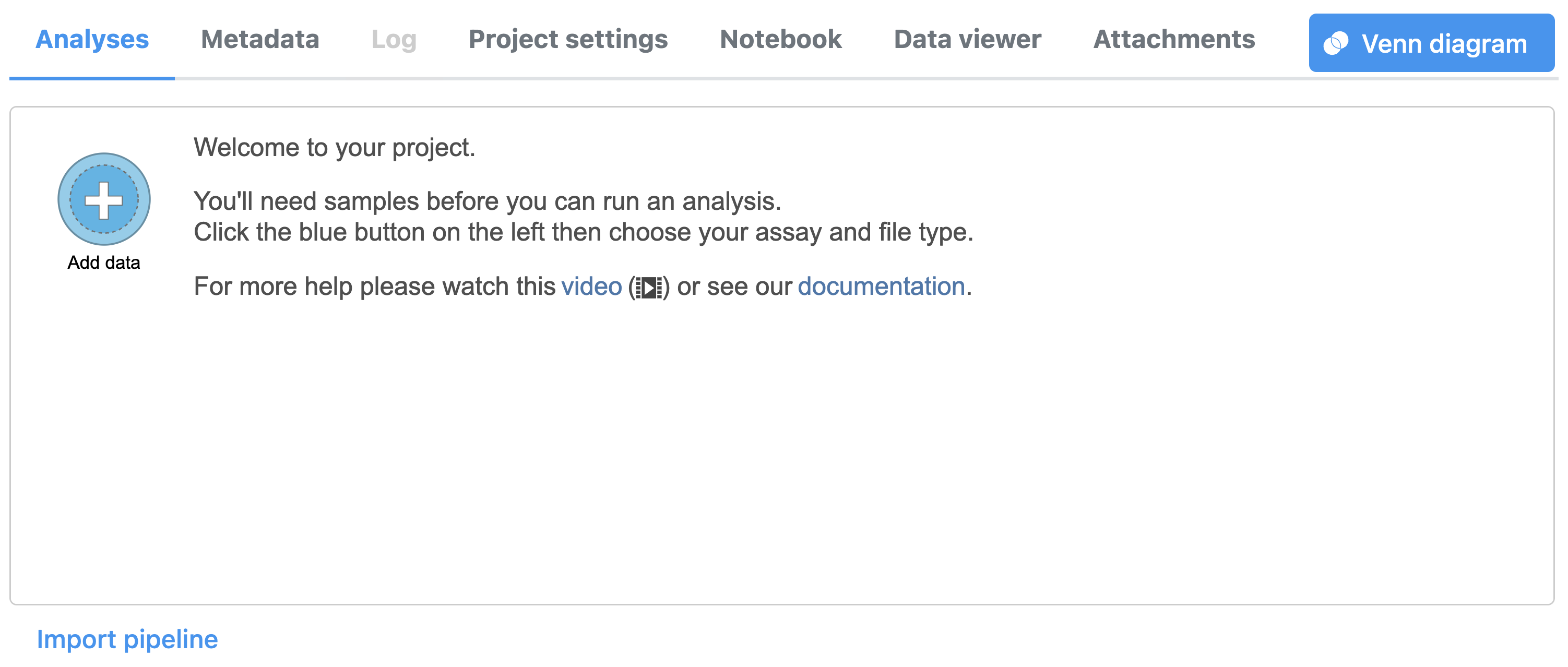
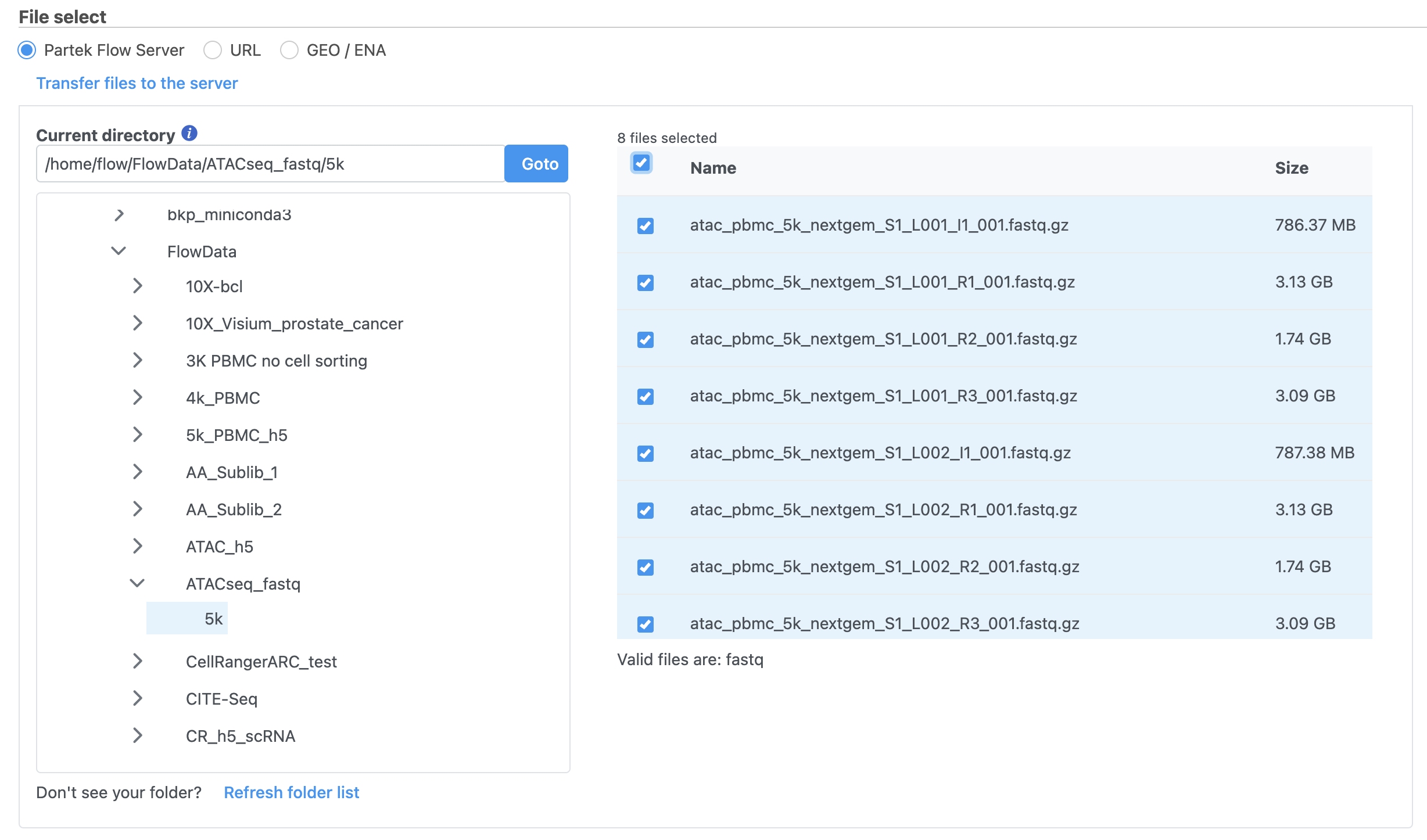
Import the FASTQ files
...
| Numbered figure captions | ||||
|---|---|---|---|---|
| ||||
|
| Numbered figure captions | ||||
|---|---|---|---|---|
| ||||
|
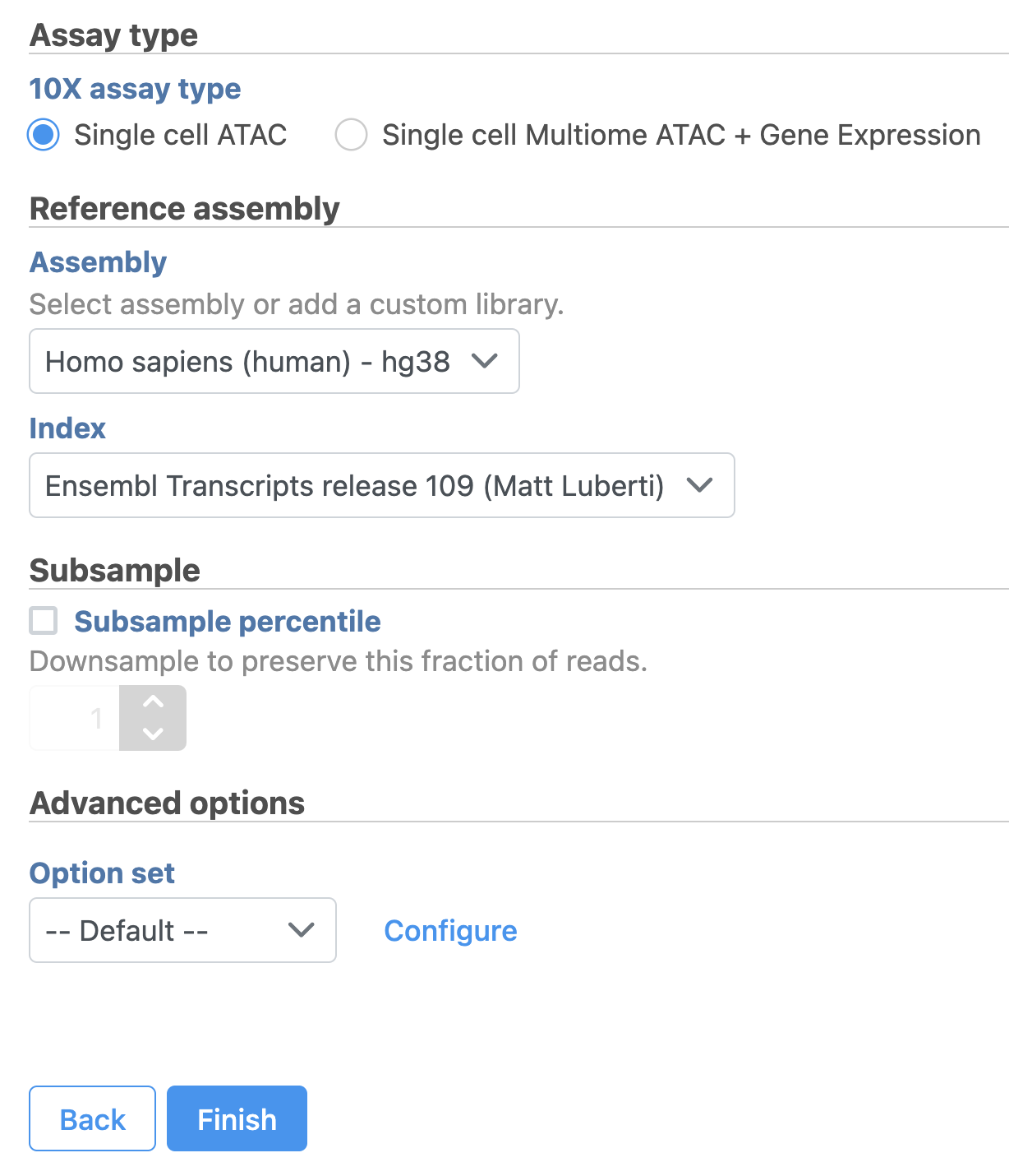
Convert FASTQ to count
...
| Numbered figure captions | ||||
|---|---|---|---|---|
| ||||
|
To learn more about how to run Cell Ranger - ATAC task in Flow, please refer to our online documentation.
...
| Numbered figure captions | ||||
|---|---|---|---|---|
| ||||
|
QA/QC
An important step in analyzing single cell ATAC data is to filter out low quality cells. A few examples of low-quality cells are doublets, cells with a low TSS enrichment score, cells with a high proportion of reads mapping to the genomic blacklist regions, or cells with too few reads to be analyzed. Users are able to do this in Partek Flow using the Single cell QA/QC task.
...
| Numbered figure captions | ||||
|---|---|---|---|---|
| ||||
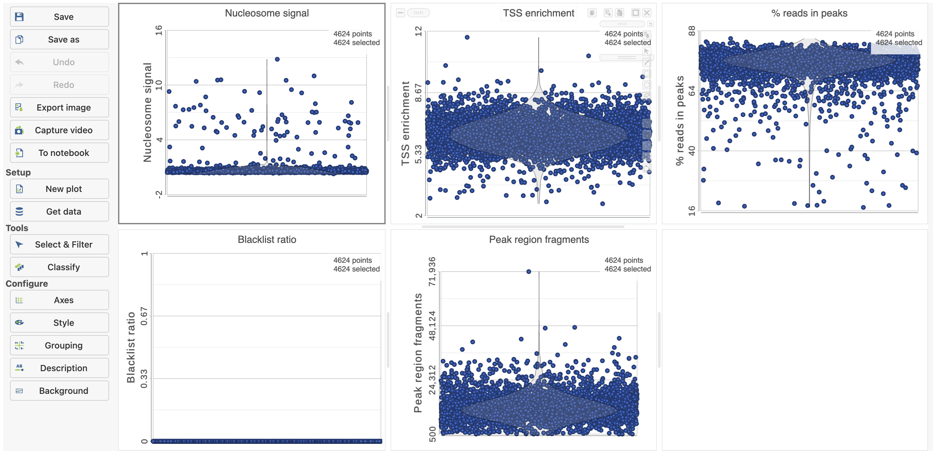 |
The Single cell QA/QC report includes interactive violin plots showing the value of every cell in the project on several quality measures (Figure 6).
...
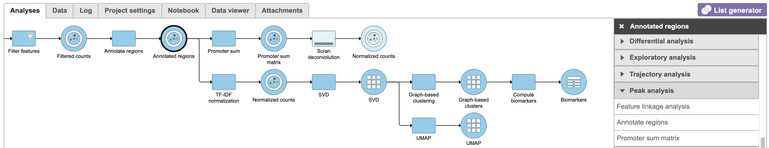
The input for Annotate peaks is a Peaks type data node.
- Click a Peaks the Filtered features data node
- Click the Peak analysis section in the toolbox
- Click Annotate regions
- Set the Genomic overlaps parameter
...
| Numbered figure captions | ||||
|---|---|---|---|---|
| ||||
|
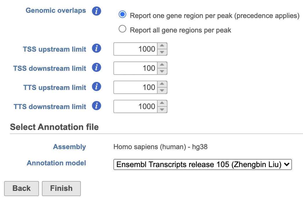
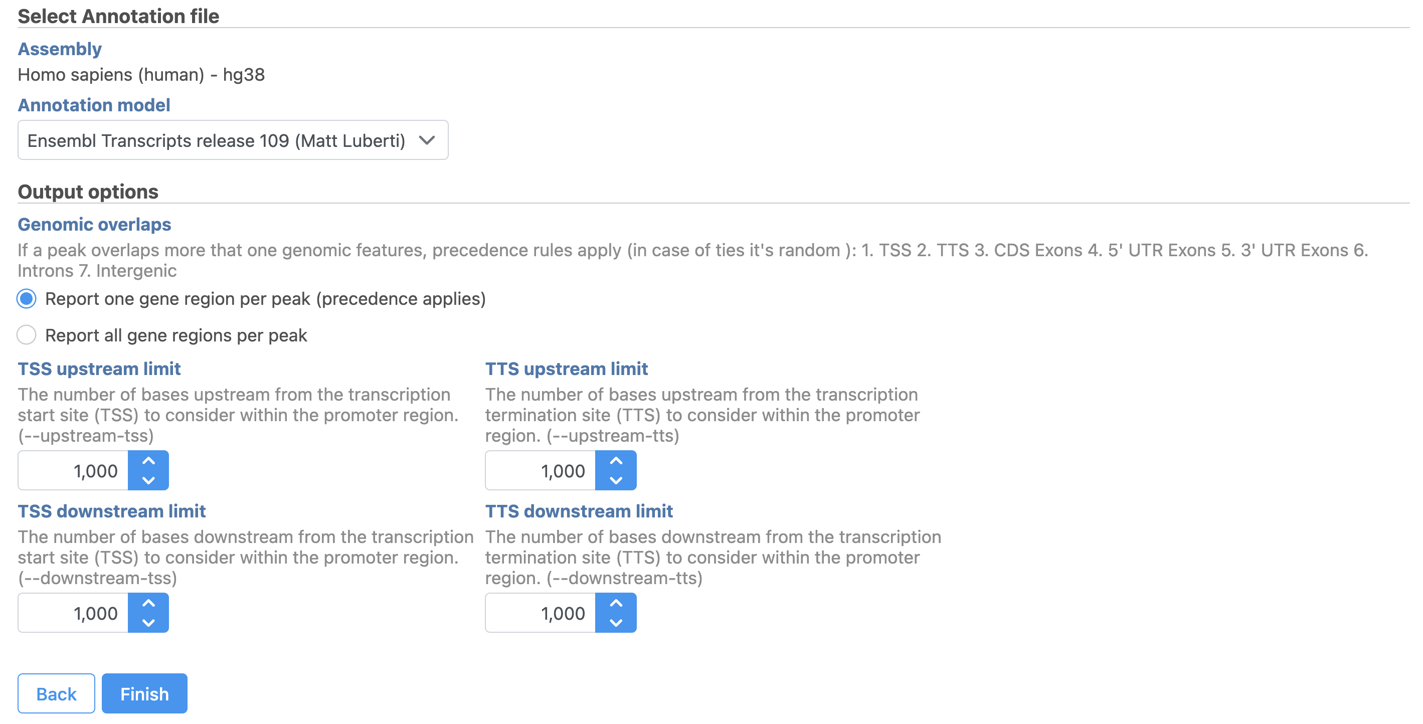
Users are able to define the transcription start site (TSS) and transcription termination site (TTS) limit in the unit of bp.
...
Latent semantic indexing (LSI) was first introduced for the analysis of scATAC-seq data by Cusanovich et al. 2018[2]. LSI combines steps of frequency-inverse document frequency (TF-IDF) normalization followed by singular value decomposition (SVD). Partek® Flow® wrapped Signac's TF-IDF normalization for single cell ATAC-seq dataset. It is a two-step normalization procedure that both normalizes across cells to correct for differences in cellular sequencing depth, and across peaks to give higher values to more rare peaks[3].
...
| Numbered figure captions | ||||
|---|---|---|---|---|
| ||||
|
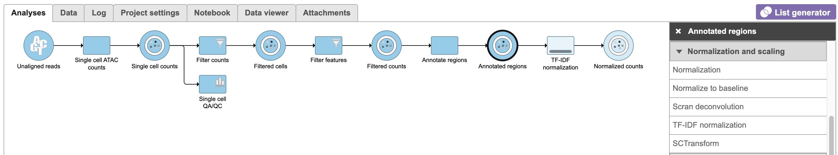
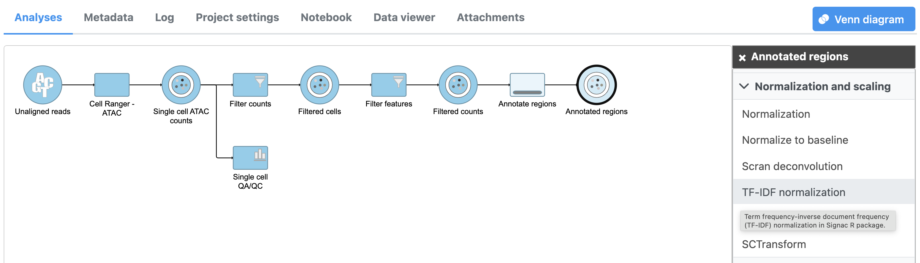
To run TF-IDF normalization,
- Click a single Single cell counts data node, in this case the Annotated regions node
- Click the Normalization and scaling section in the toolbox
- Click TF-IDF normalization
...
| Numbered figure captions | ||||
|---|---|---|---|---|
| ||||
|
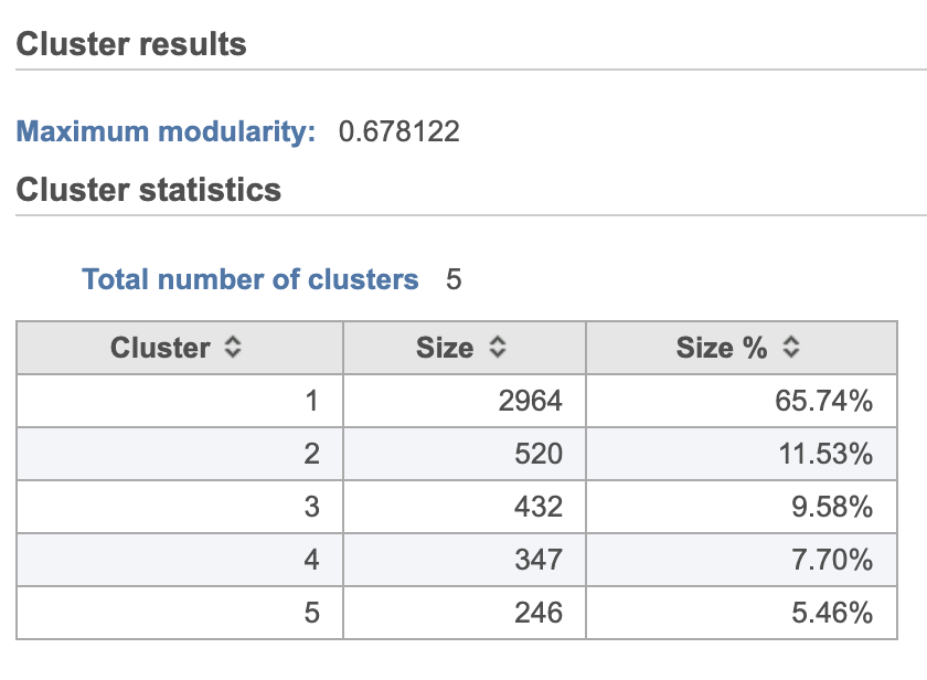
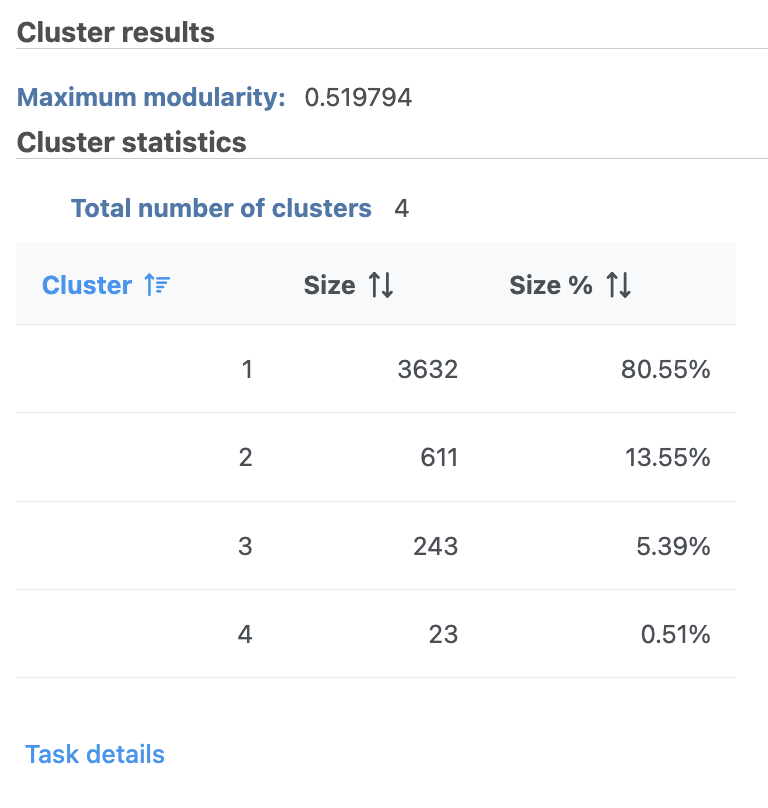
Graph-based clustering
...
| Numbered figure captions | ||||
|---|---|---|---|---|
| ||||
|
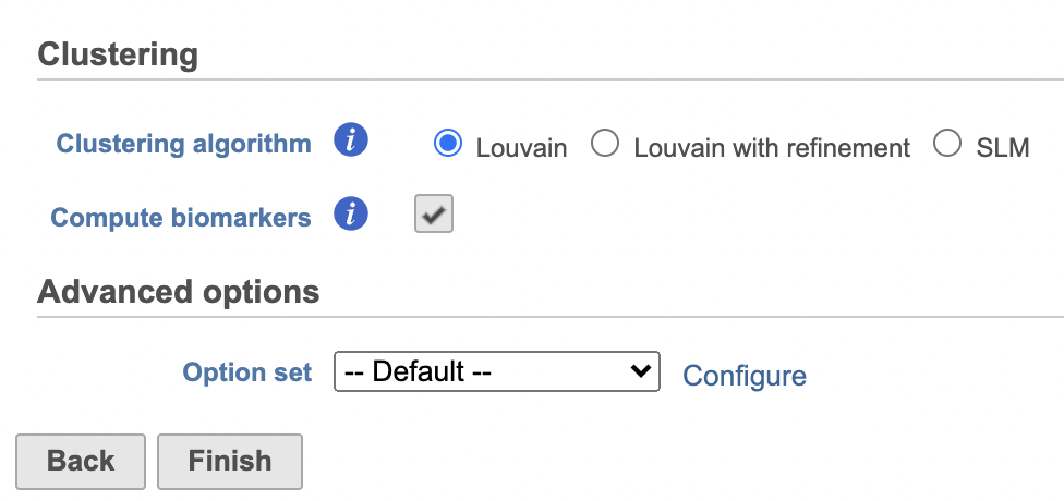
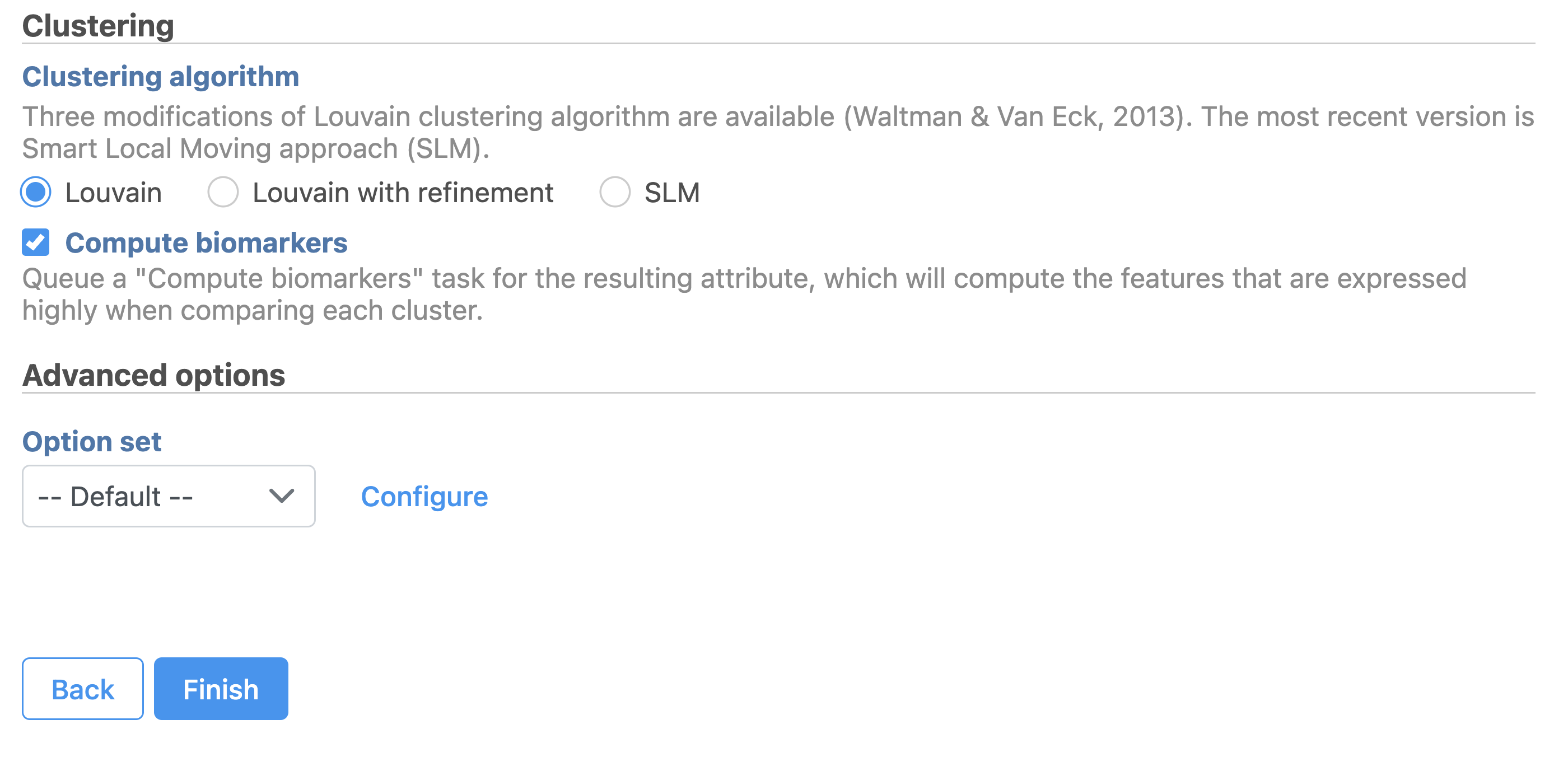
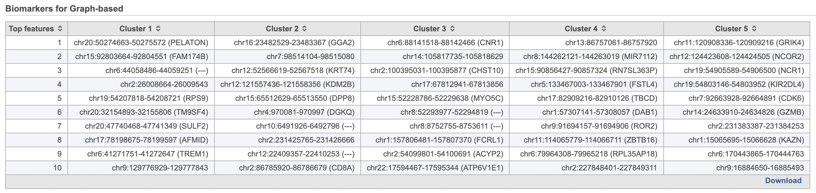
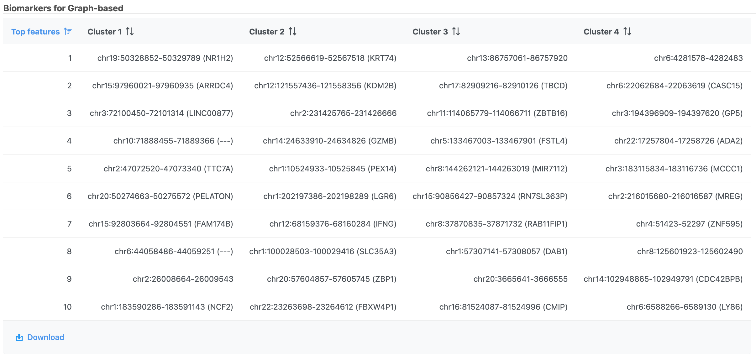
A new Graph-based clusters data and a Biomarkers data node will be generated.
...
| Numbered figure captions | ||||
|---|---|---|---|---|
| ||||
|
| Numbered figure captions | ||||
|---|---|---|---|---|
| ||||
|
UMAP
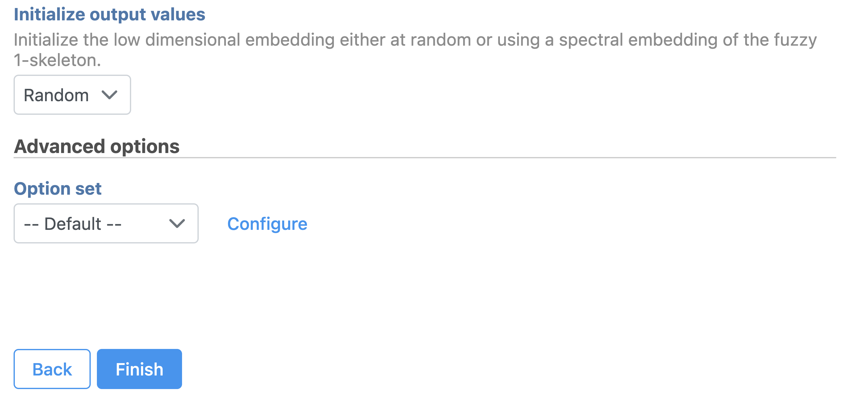
Similar to t-SNE, Uniform Manifold Approximation and Projection (UMAP) is a dimensional reduction technique. UMAP aims to preserve the essential high-dimensional structure and present it in a low-dimensional representation. UMAP is particularly useful for visually identifying groups of similar samples or cells in large high-dimensional data sets.
...
| Numbered figure captions | ||||
|---|---|---|---|---|
| ||||
|
Promoter sum matrix
...
| Numbered figure captions | ||||
|---|---|---|---|---|
| ||||
|
Classifying cells
...
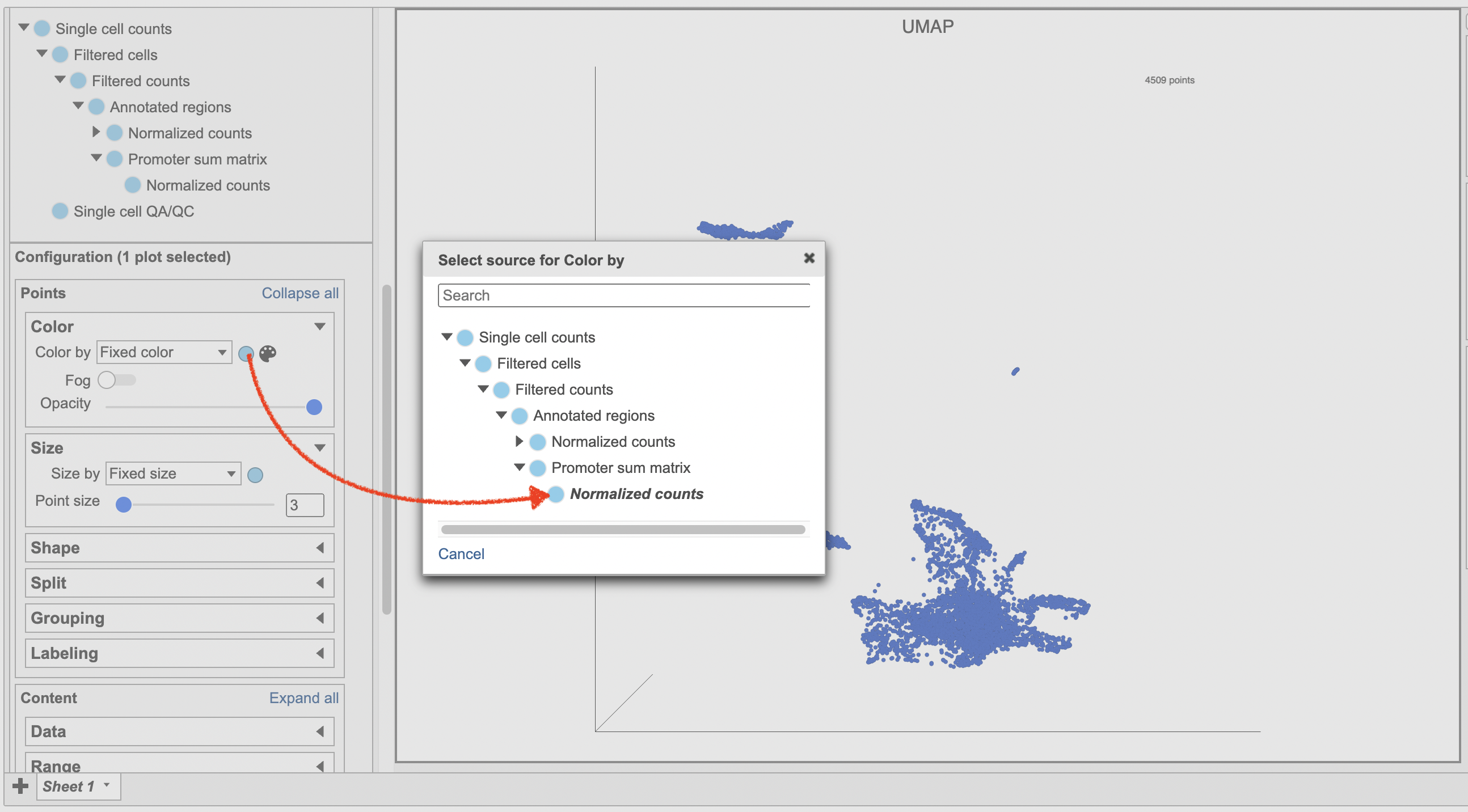
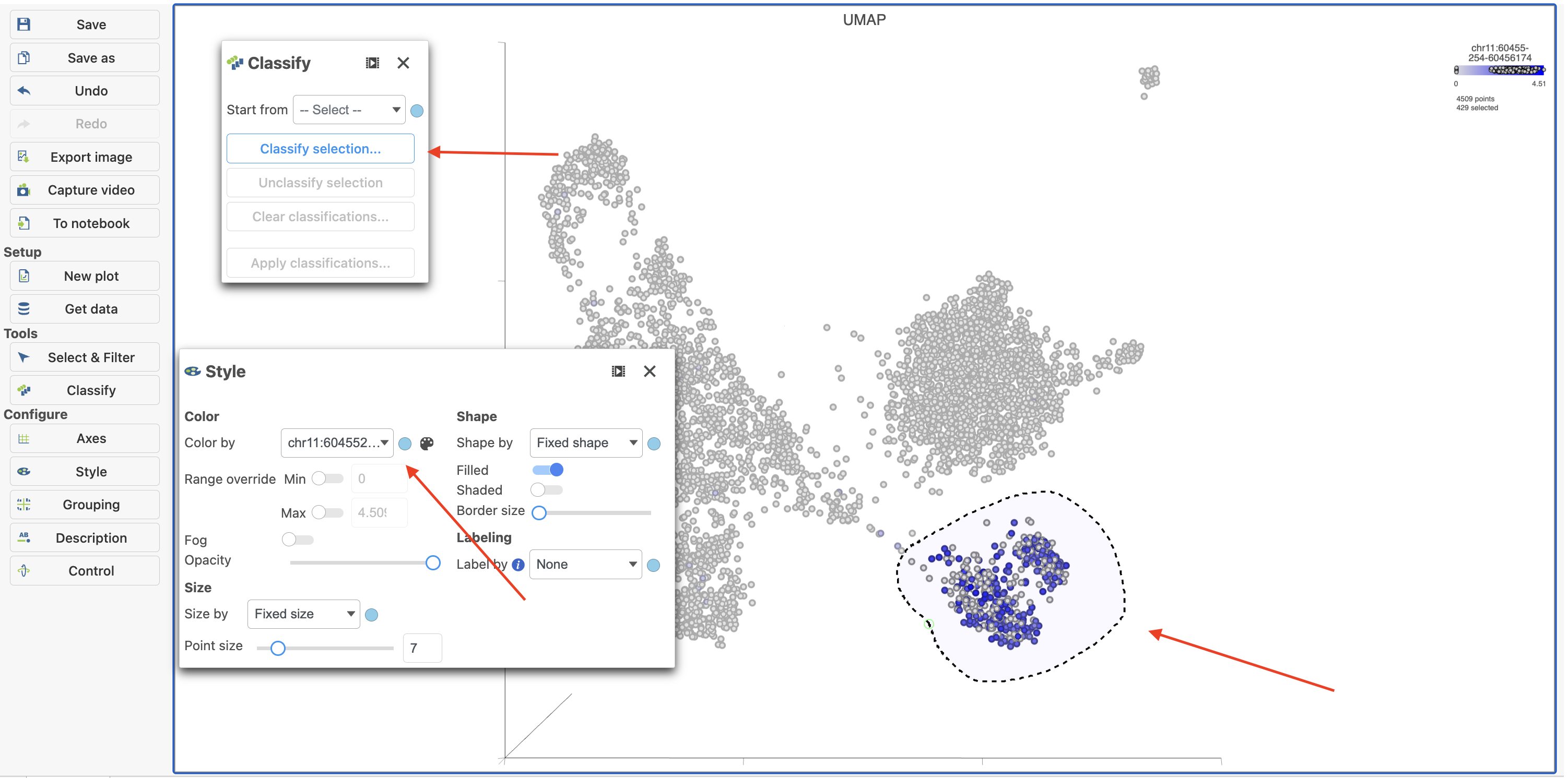
- Make sure the right data source has been selected. For scATAC-seq data, it shall be the normalized counts of promoter sum values in most cases (Figure 17)
- Set Color by in the Style configuration to the normalized counts node
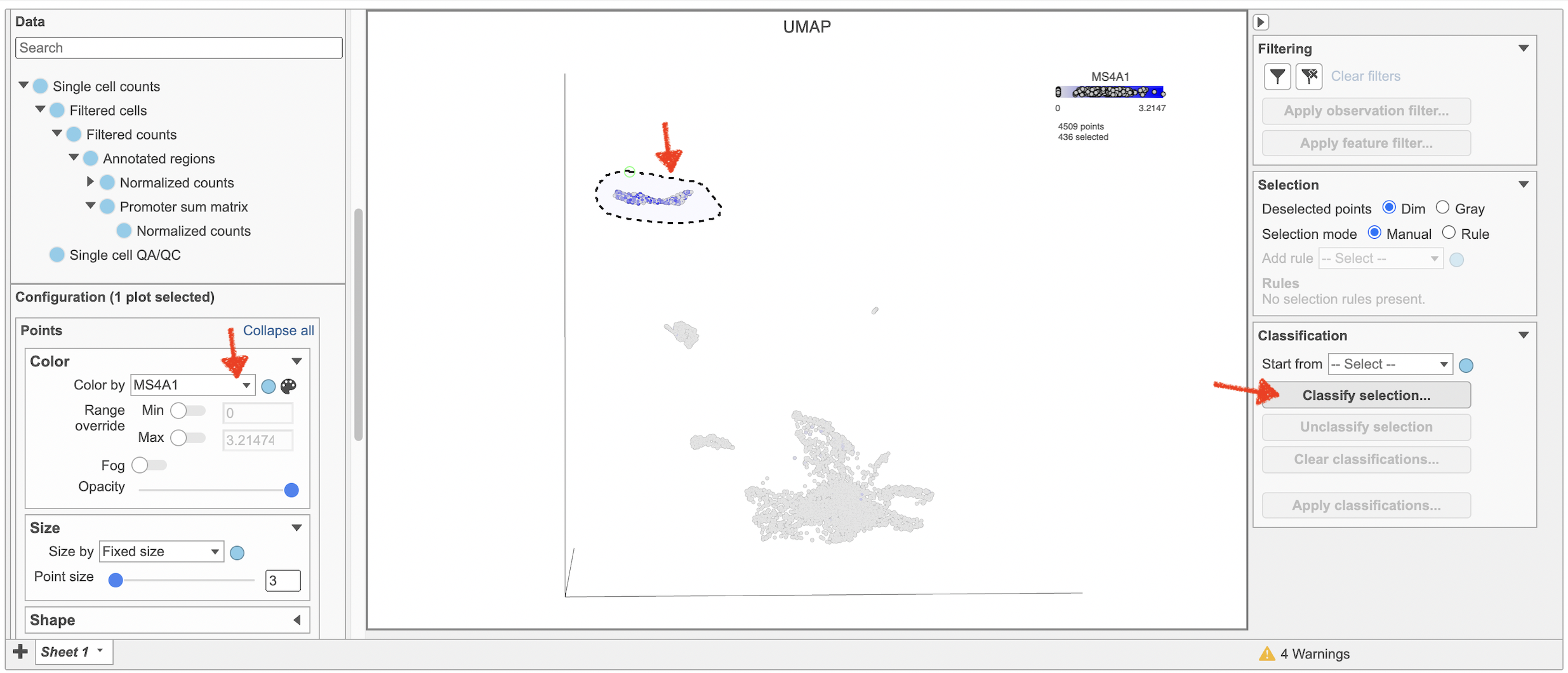
- Type MS4A1 in the search box and select it. Rotate the 3D plot if you need to see this cluster more clearly.
- Click Click
 to activate Lasso mode
 - Draw a lasso around the cluster of MS4A1-expressing cells
- Click Classify selection under Tools in the left panel
- Type B cells for the Name
- Click Save (Figure 18)
...
| Numbered figure captions | ||||
|---|---|---|---|---|
| ||||
|

| Numbered figure captions | ||||
|---|---|---|---|---|
| ||||
|
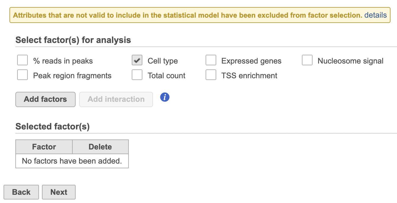
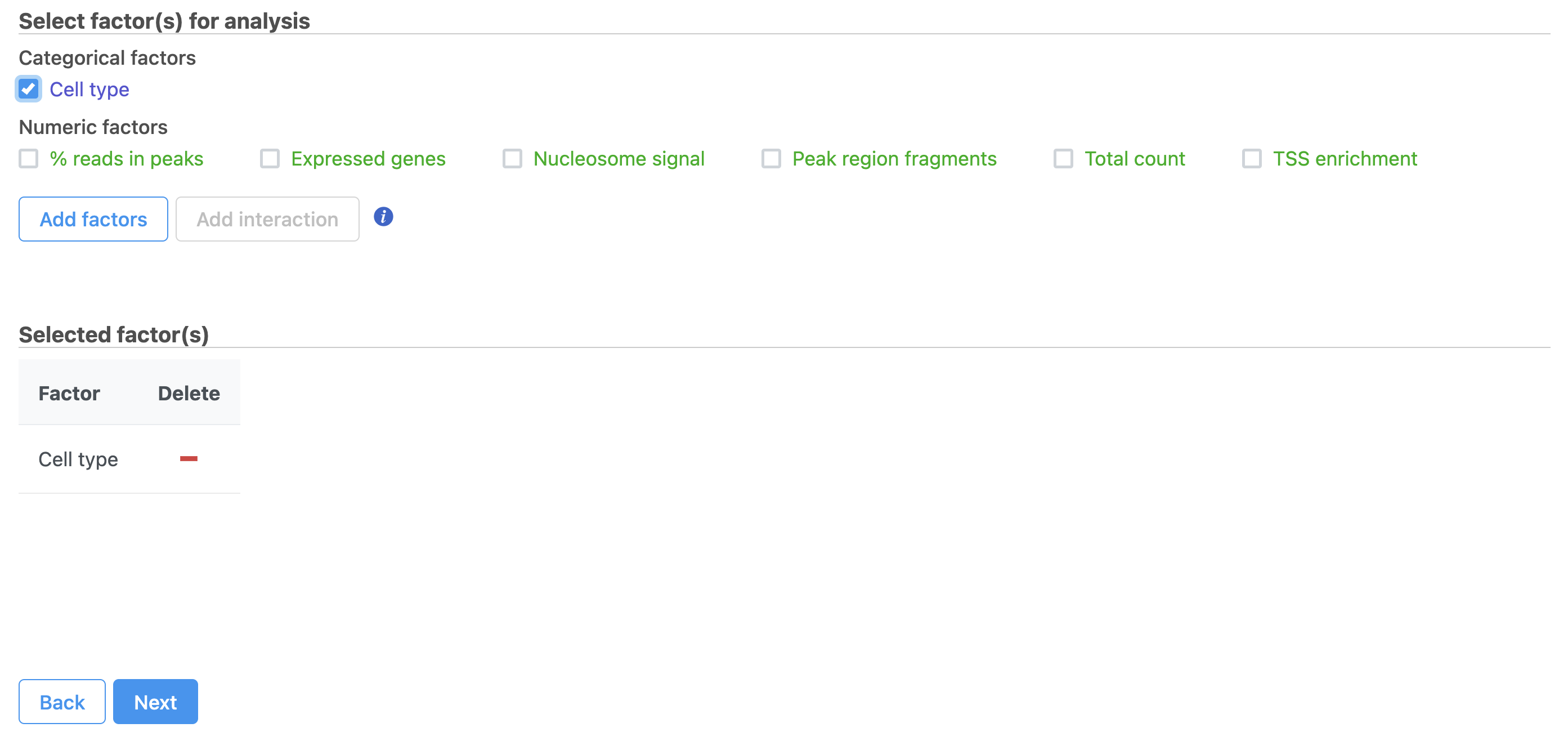
Differential analysis
...
| Numbered figure captions | ||||
|---|---|---|---|---|
| ||||
|
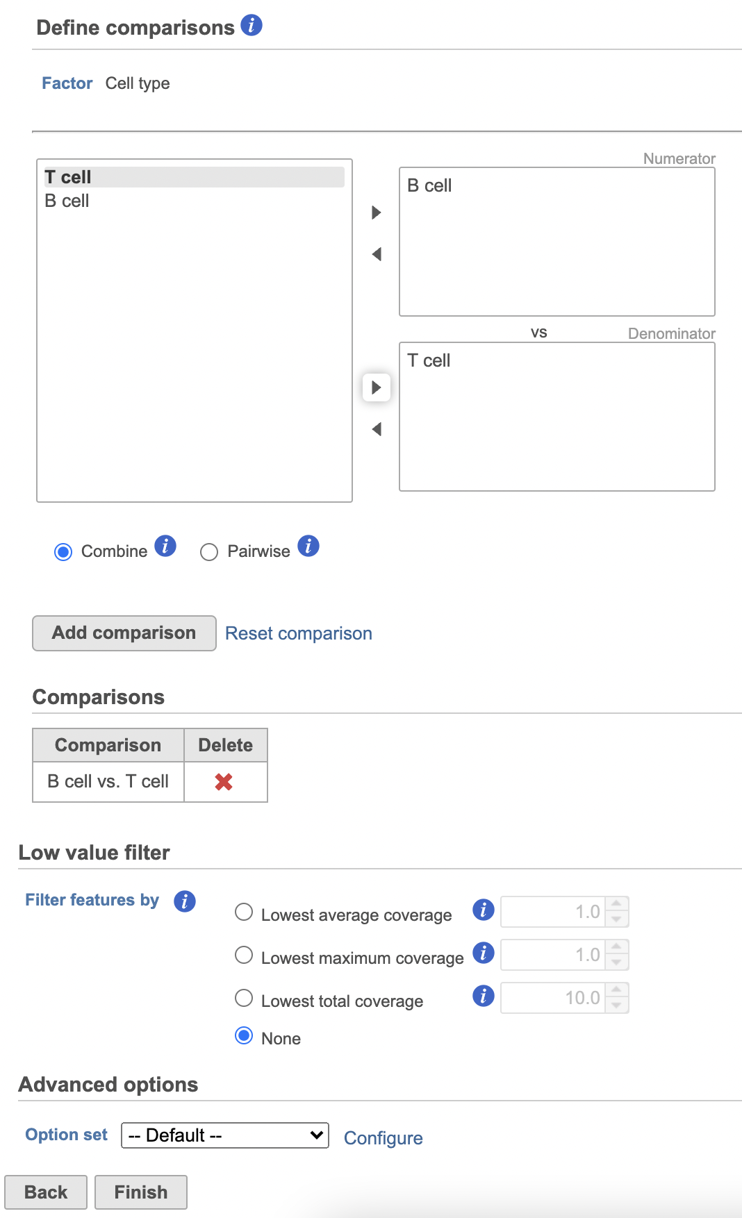
- Click Next
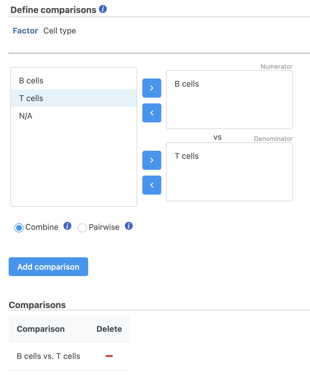
- Define comparisons between factor or interaction levels (Figure 20)
- Click Add comparison to add the comparison to the Comparisons table.
- Click Finish to run the statistical test as default
| Numbered figure captions | ||||
|---|---|---|---|---|
| ||||
|
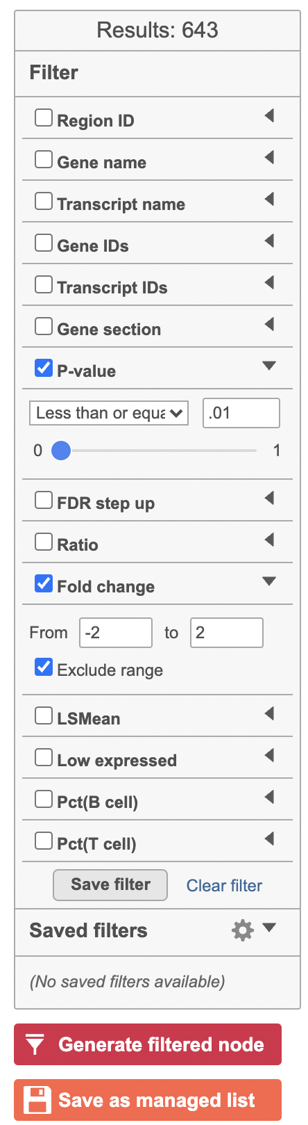
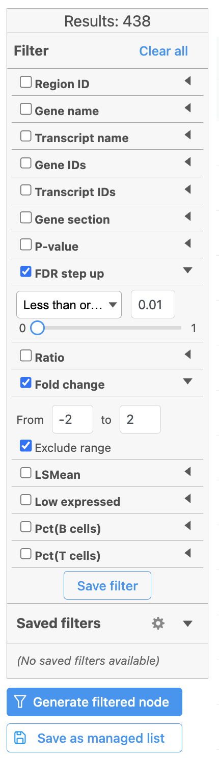
Hurdle model produces a Feature list task node. The results table and options are the same as the GSA task report except the last two columns. The percentage of cells where the feature is detected (value is above the background threshold) in different groups (Pct(group1), Pct(group2)) are calculated and included in the Hurdle model report.
...
| Numbered figure captions | ||||
|---|---|---|---|---|
| ||||
  |
Once we have filtered a list of differentially expressed genes, we can visualize these genes by generating a heatmap, or perform the Gene set enrichment analysis and motif detection.
...
Overview
Content Tools