For your convenience, here is a video showing the below steps.  

This guide illustrates how to process FASTQ files produced using the 10x Genomics Chromium Single Cell ATAC assay to obtain a Single cell counts data node, which is the starting point for analysis of single-cell ATAC experiments.

If you are new to Partek® Flow®, please see Getting Started with Your Partek Flow Hosted Trial for information about data transfer and import and Creating and Analyzing a Project for information about the Partek Flow user interface.  

This tutorial uses a 10X 5k PBMC dataset if you would like to follow along exactly.

Transfer files and create a new project

We recommend uploading your FASTQ files (fastq.gz) to a folder on your Partek® Flow® server before importing them into a project. Data files can be transferred into Flow from the Home page by clicking the Transfer file button (Figure 1). Following the instruction In Figure 1 to complete the data transfer. Users have the option to change the Upload directory by clicking the Browse button and either select another existing directory or create a new directory. 

To create a new project, from the Home page click the New Project button; enter a project name and then click Create project. Once a new project has been created, click the Add data button in the Analyses tab. 

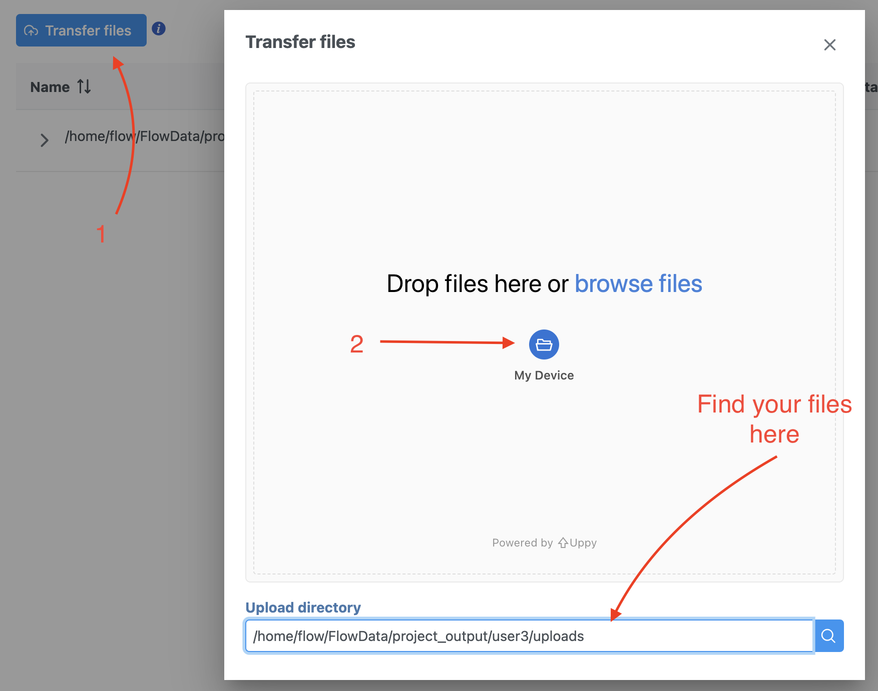
Figure 1. Transfer file in Partek Flow.

Import the FASTQ files

To proceed, click the Add data button in the Analyses tab. In the Single cell > scATAC-Seq section select fastq and click Next. The file browser interface will open (Figure 3). Select the FASTQ files using the file browser interface and push the Finish button to complete the task. Paired end reads will be automatically detected and multiple lanes for the same sample will be automatically combined into a single sample. We encourage users to include all the FASTQ files including the index files although they are optional. 

When the FASTQ files have finished importing, the Unaligned reads data node will appear in the Analyses tab.

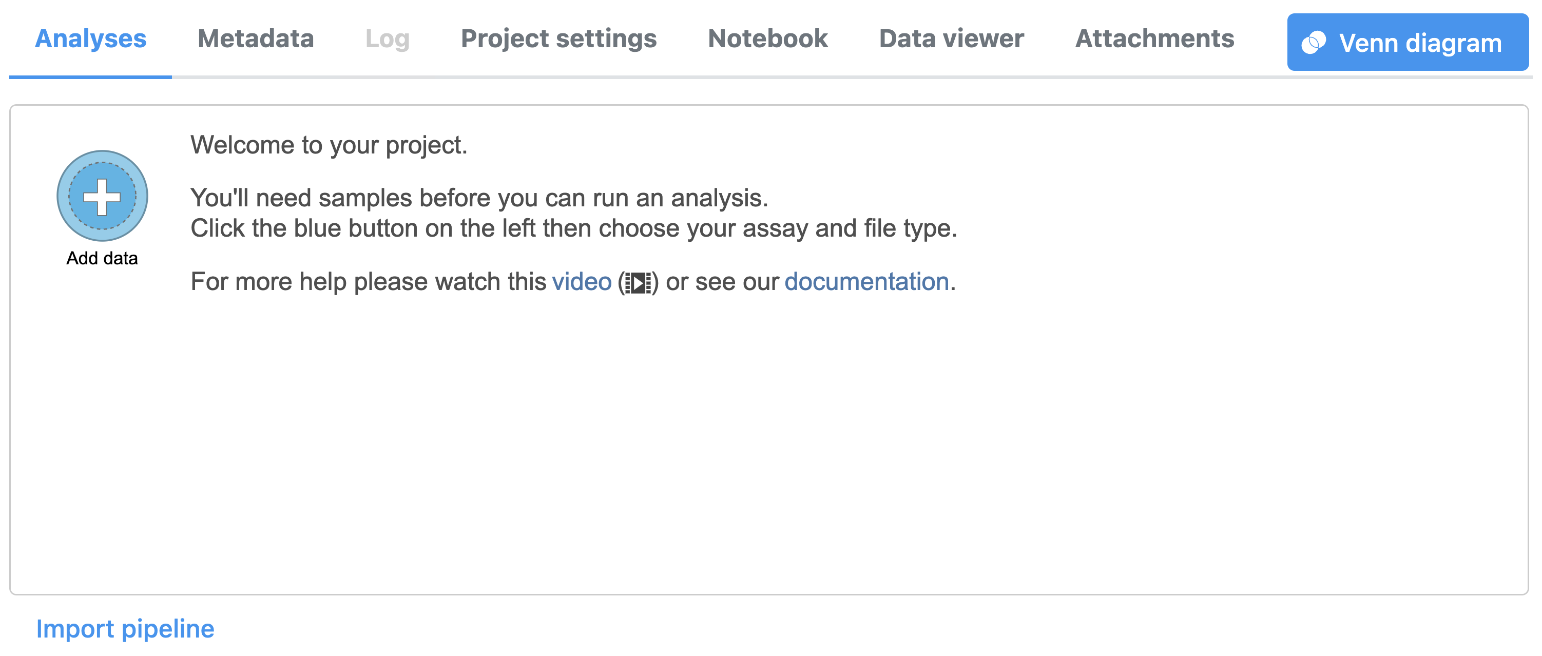
Figure 2. Data tab in Partek Flow.

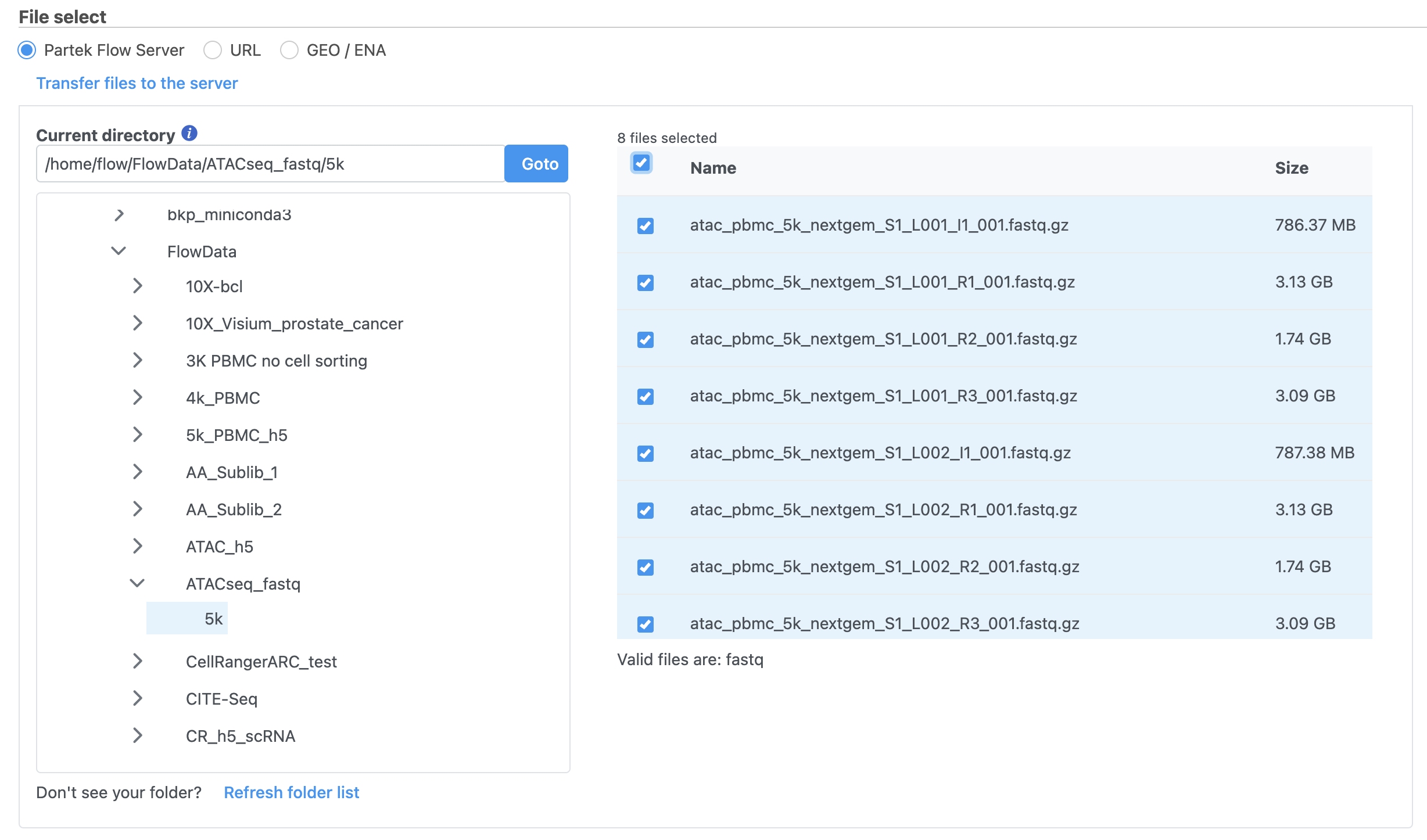
Figure 3. Input FASTQ files for scATAC-Seq data in Flow.

Convert FASTQ to count 

To deal with the single cell ATAC-seq FASTQ data, Flow® has wrapped the 'cellranger-atac count' pipeline from Cell Ranger ATAC v2.0[1]. It takes FASTQ files and performs multiple analysis simultaneously including reads filtering and alignment, barcode counting, identification of transposase cut sites, peak and cell calling, and generates the count matrix.

To run Cell Ranger - ATAC task:  

• Click the Unaligned reads data node
• Select Cell Ranger - ATAC in the 10x Genomics section in the task menu on the right
• Select Single cell ATAC in Assay type for ATAC-Seq data only
• Choose the proper Reference assembly for the data (you may have to create the reference)
• Press the Finish button to run the task with default settings (Figure 4)
  
  

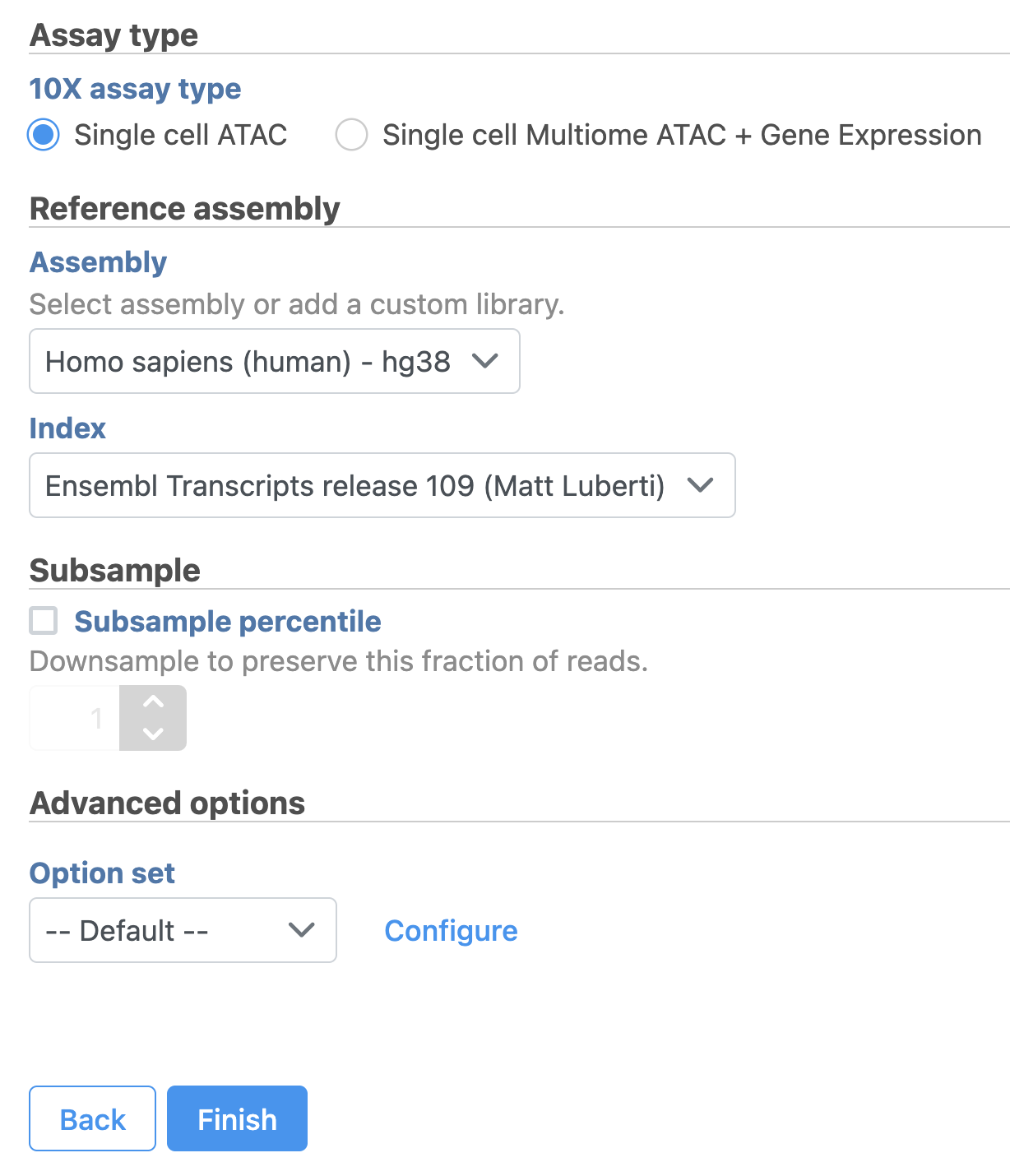
Figure 4. Convert FASTQ by Cell Ranger - ATAC task in Flow.

To learn more about how to run Cell Ranger - ATAC task in Flow, please refer to our online documentation.

The output of the count matrix then becomes the starting point for downstream analysis for scATAC-seq data in Flow (Figure 5). 

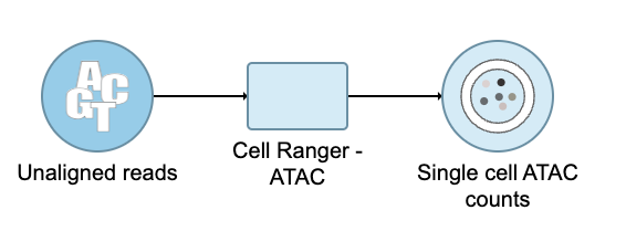
Figure 5. Single cell QA/QC task for scATAC-Seq data in Flow.

QA/QC

An important step in analyzing single cell ATAC data is to filter out low quality cells. A few examples of low-quality cells are doublets, cells with a low TSS enrichment score, cells with a high proportion of reads mapping to the genomic blacklist regions, or cells with too few reads to be analyzed. Users are able to do this in Partek Flow using the Single cell QA/QC task. 

• Click on the Single cell counts node
• Click on the QA/QC section in the task menu
• Click on Single cell QA/QC 

A task node, Single cell QA/QC, is produced. Initially, the node will be semi-transparent to indicate that it has been queued, but not completed. A progress bar will appear on the Single cell QA/QC task node to indicate that the task is running (Figure 5).

• Click the Single cell QA/QC node once it finishes running 
• Click Task report in the task menu
  
  

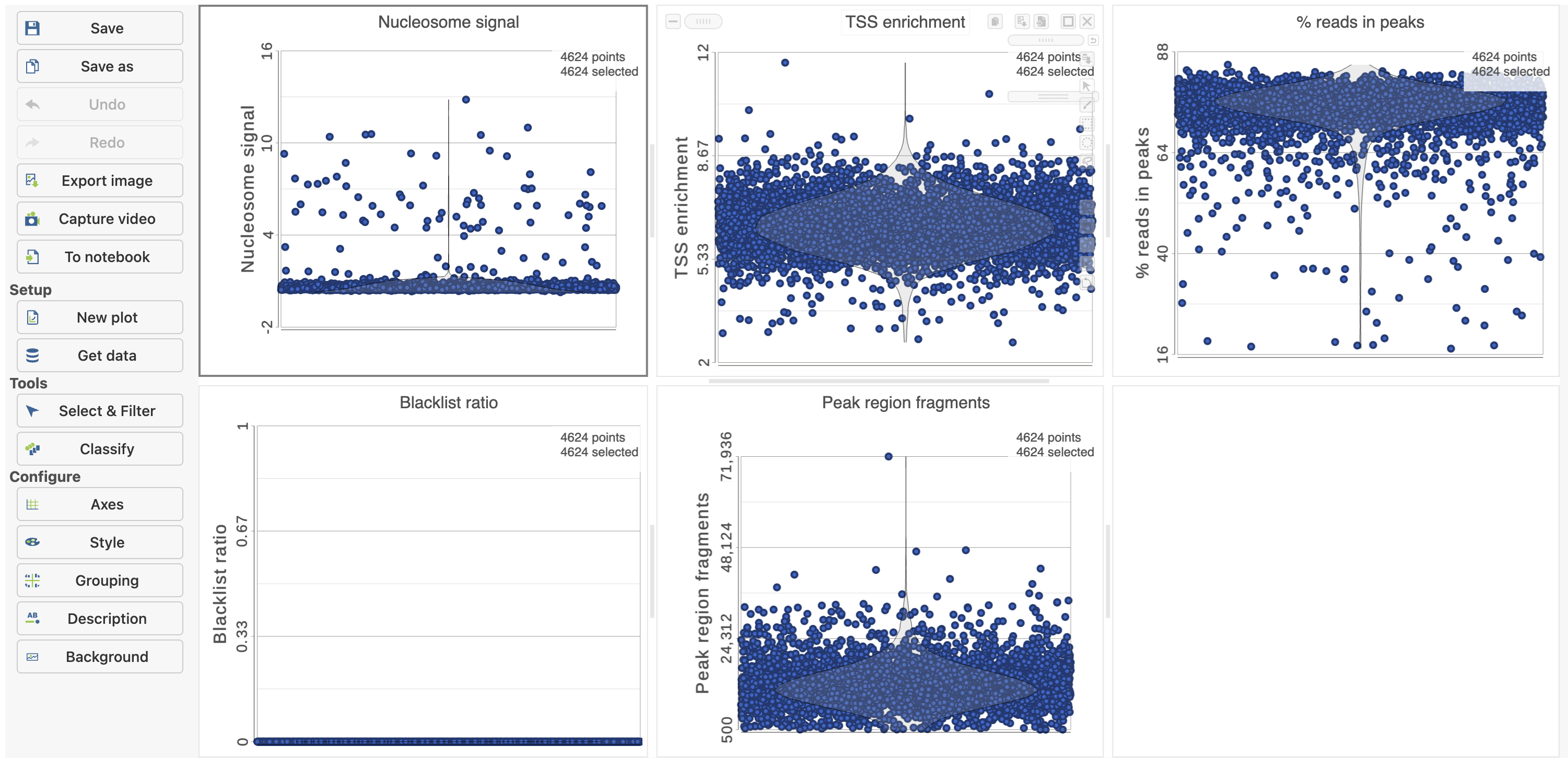
Figure 6. QA/QC task report for scATAC - Seq data in Flow.

The Single cell QA/QC report includes interactive violin plots showing the value of every cell in the project on several quality measures (Figure 6).

There are five plots: Nucleosome signal, TSS enrichment, % reads in peaks, Blacklist ratio, and Peak region fragments. Each point on the plots is a cell and the violins illustrate the distribution of values for the y-axis metric. Cells can be filtered either by clicking and dragging to select a region on one of the plots or by setting thresholds using the filters below the plots. Here, we will apply a filter for the number of read counts. The plot will be shaded to reflect the filter. Cells that are excluded will be shown as black dots on both plots.

Descriptions of QC metrics:

Nucleosome signal: calculated per single cell, which quantifies the approximate ratio of mononucleosomal to nucleosome-free fragments. The histogram of DNA fragment sizes (determined from the paired-end sequencing reads) should exhibit a strong nucleosome banding pattern which corresponds to the length of DNA wrapped around a single nucleosome.

TSS enrichment: Transcriptional start site (TSS) enrichment score. The ENCODE project has defined an ATAC-seq targeting score based on the ratio of fragments centered at the TSS to fragments in TSS-flanking regions (see https://www.encodeproject.org/data-standards/terms/). Poor ATAC-seq experiments typically will have a low TSS enrichment score.

Peak region fragments: total number of fragments in peaks which is a measure of cellular sequencing depth/complexity. Cells with very few reads may need to be excluded due to low sequencing depth. Cells with extremely high levels may represent doublets, nuclei clumps, or other artifacts.

% reads in peaks: Represents the fraction of all fragments that fall within ATAC-seq peaks. Cells with low values (i.e. <15-20%) often represent low-quality cells or technical artifacts that should be removed. Note that this value can be sensitive to the set of peaks used.

Blacklist ratio: The ENCODE project has provided a list of blacklist regions, representing reads which are often associated with artifactual signals. Cells with a high proportion of reads mapping to these areas (compared to reads mapping to peaks) often represent technical artifacts and should be removed.  

Filter cells

To filter out low quality cells (Figure 7), 

• Open the Select & Filter menu
• Set the filters on nucleosome signal < 4; Peak region fragment 500-30000; leave the rest as they are
• Click the filter icon and Apply observation filter to run the Filter cells task on the first Single cell ATAC counts data node, it generates a Filtered cells node

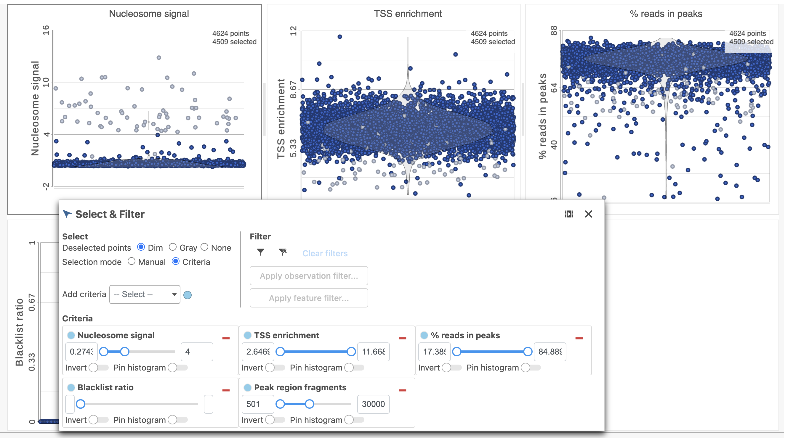
Figure 7. Filter low quality cells in Partek Flow.

Filter features

Another common task is to filter the data to include only informative features. Partek Flow has a wide variety of flexible filtering options. 

Filter features task can be invoked from any counts or single cell data node. Noise Reduction and Statistics Based filters take each feature and perform the specified calculation across all the cells. The filter is applied to the values in the selected data node and the output is a filtered version of the input data node. 

In the task dialog, click the check box to activate one or more of the filter types, configure the filter(s), and click Finish to run (Figure 8). 

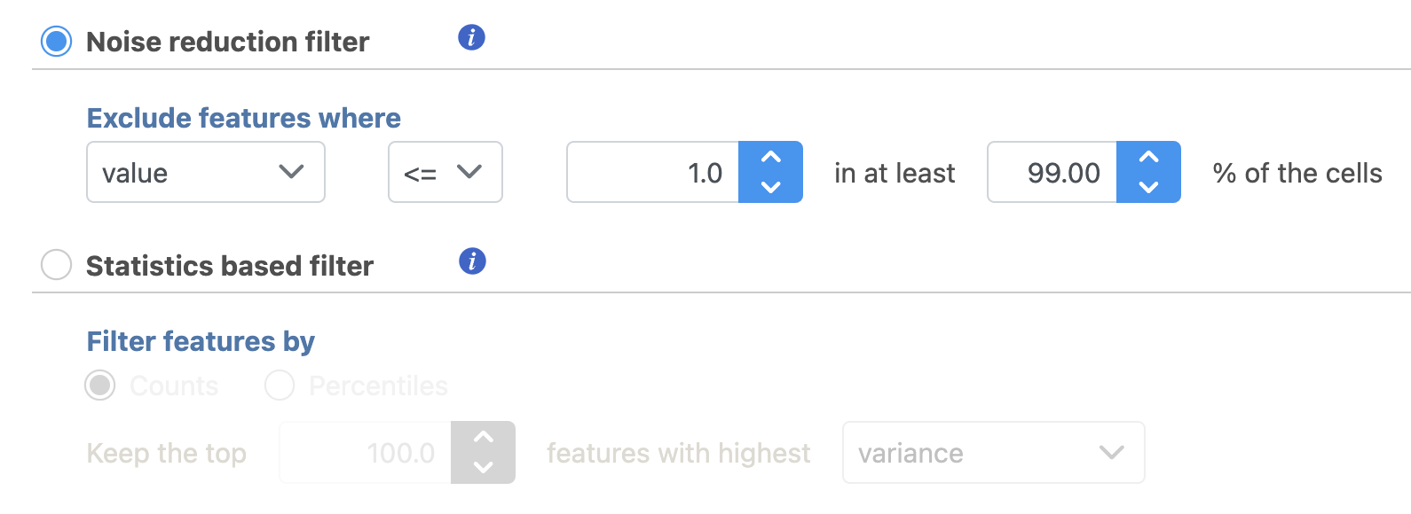
Figure 8. Filter features in Partek Flow.

Annotate regions

To understand the importance of enriched regions in regulating gene expression, Flow uses Annotate regions task to add information about overlapping or nearby genomic features. That gives regulatory context for enriched regions.

The input for Annotate peaks is a Peaks type data node. 

• Click the Filtered features data node
• Click the Peak analysis section in the toolbox
• Click Annotate regions
• Set the Genomic overlaps parameter

The Genomics overlaps parameter lets you choose one of two options (Figure 9).

• Report one gene region per peak (precedence applies) chooses one gene section for each peak using the precedence order to settle cases where more than one gene section overlaps a peak. The order of precedence is TSS, TTS, CDS Exon, 5' UTR Exon, 3' UTR Exon, Intron, Intergenic.
• Report all gene regions per peak creates a row for each gene section that overlaps a peak in the task report. 

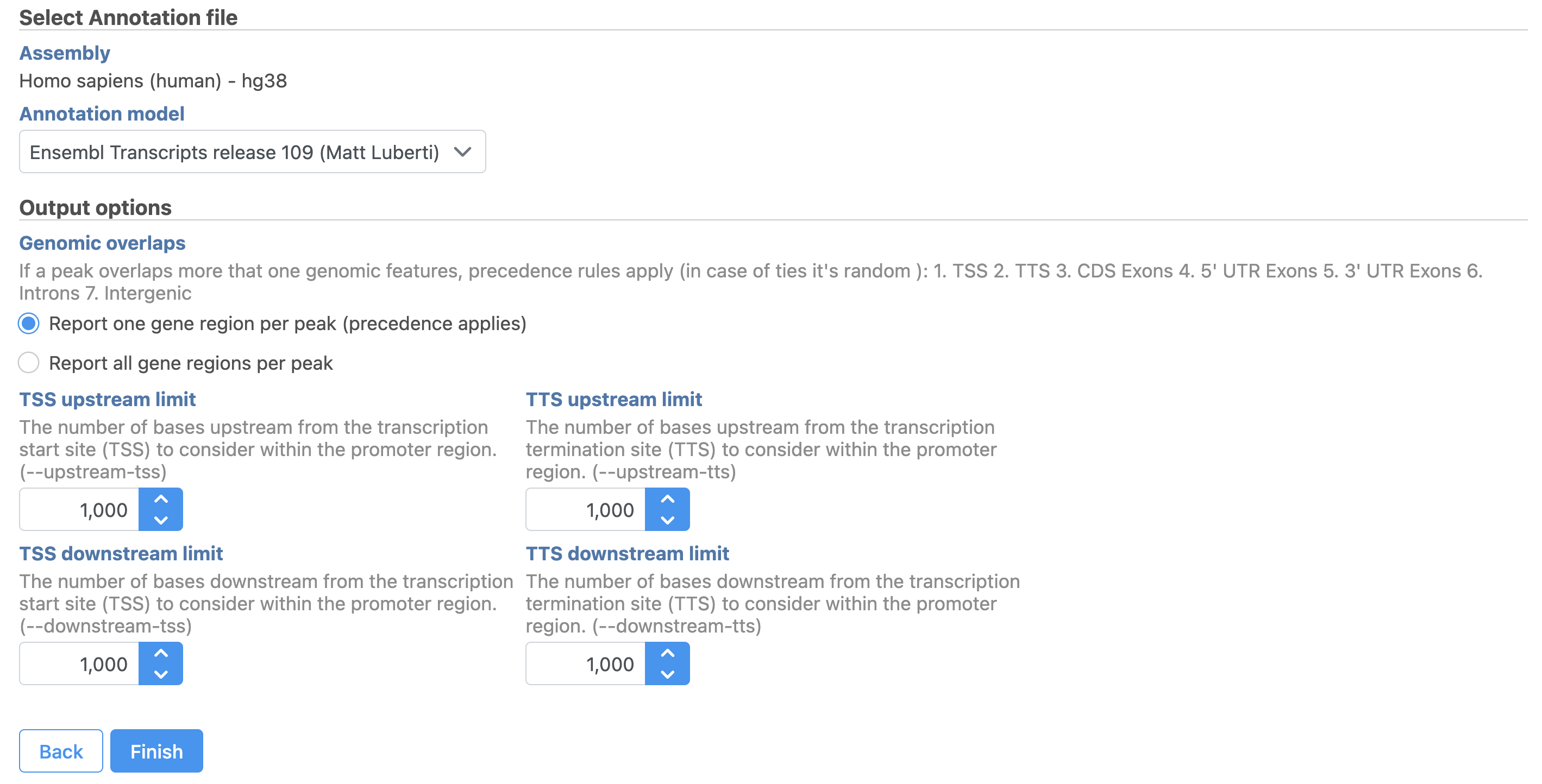
Figure 9. Annotate regions in Partek Flow.

Users are able to define the transcription start site (TSS) and transcription termination site (TTS) limit in the unit of bp.

• Choose a gene/feature annotation from the drop-down menu
• Click Finish to run

TF-IDF (frequency-inverse document frequency) normalization

Latent semantic indexing (LSI)  was first introduced for the analysis of scATAC-seq data by Cusanovich et al. 2018[2]. LSI combines steps of frequency-inverse document frequency (TF-IDF) normalization followed by singular value decomposition (SVD). Partek® Flow® wrapped Signac's TF-IDF normalization for single cell ATAC-seq dataset. It is a two-step normalization procedure that both normalizes across cells to correct for differences in cellular sequencing depth, and across peaks to give higher values to more rare peaks[3].

TF-IDF normalization in Flow can be invoked in Normalization and scaling section by clicking any single cell counts data node (Figure 10).

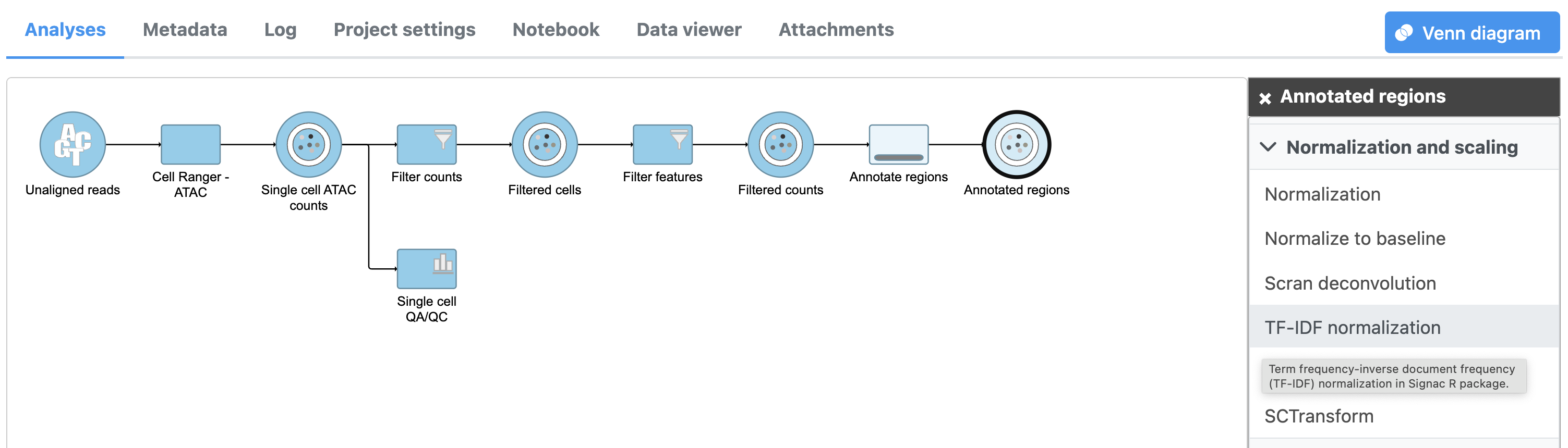
Figure 10. TF-IDF normalization for scATAC-Seq in Flow.

To run TF-IDF normalization, 

• Click a Single cell counts data node, in this case the Annotated regions node
• Click the Normalization and scaling section in the toolbox
• Click TF-IDF normalization

The output of TF-IDF normalization is a new data node that has been normalized by log(TF x IDF).

SVD (singular value decomposition )

Singular value decomposition (SVD) will be applied to TF-IDF output in scATAC-Seq data. It returns a reduced dimension representation of a matrix. Although SVD and Principal components analysis (PCA) are two different techniques, the SVD has a close connection to PCA. Because PCA is simply an application of the SVD.  For users who are more familiar with scRNA-Seq, you can think of SVD as analogous to the output of PCA. And similarly, the statistical interpretation of singular values is in the form of variance in the data explained by the various components.

To run SVD task, 

• Click a Normalized counts data node
• Click the Exploratory analysis section in the toolbox
• Click SVD

The GUI is simple and easy to understand. The SVD dialog is only asking to select the number of singular values to compute (Figure 11).  By default 100 singular values will be computed if users don't want to compute all of them.  However, the number could be adjusted manually or typed in directly.  Simply click the Finish button if you want to run the task as default.

The task report for SVD is similar to PCA. Its output will be used for downstream analysis and visualization, including Harmony and WNN.

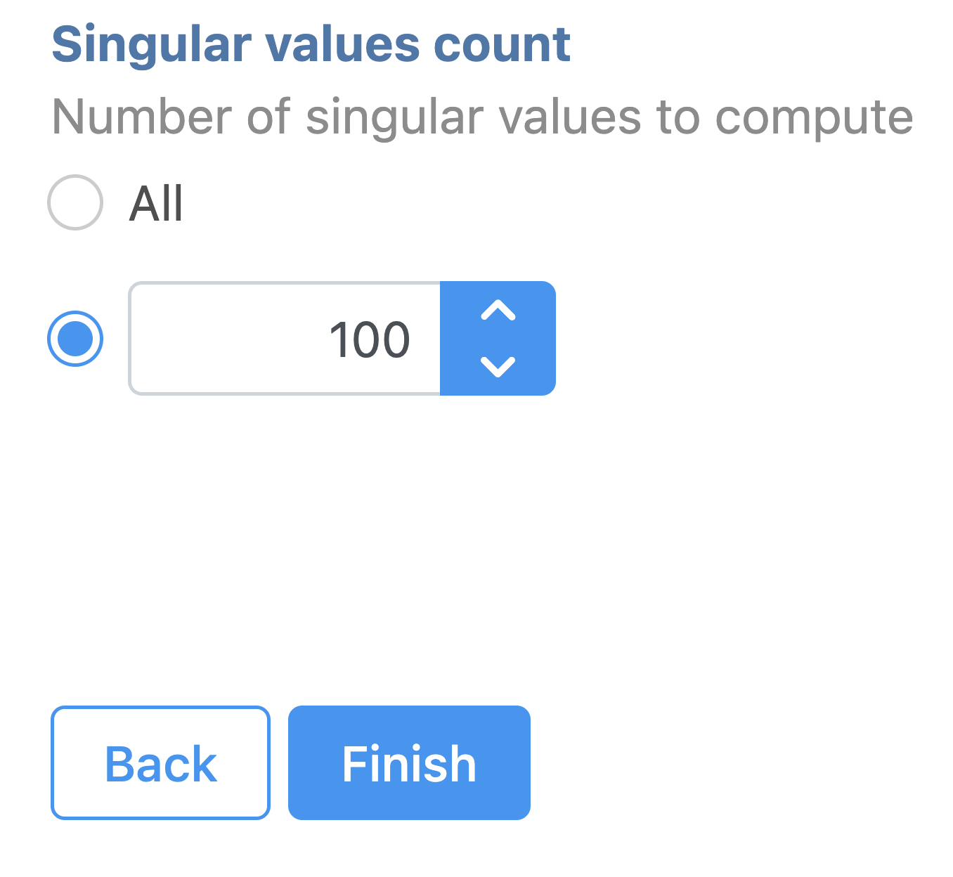
Figure 11. SVD task configuration dialog in Partek Flow.

Graph-based clustering

Graph-based clustering (Figure 12) identifies groups of similar cells using SVD values as the input. By including the informative SVDs, noise in the data set is excluded, improving the results of clustering. 

• Click the SVD output
• Click Exploratory analysis in the task menu
• Click Graph-based clustering 
• Check Compute biomarkers
• Click Finish to run as default

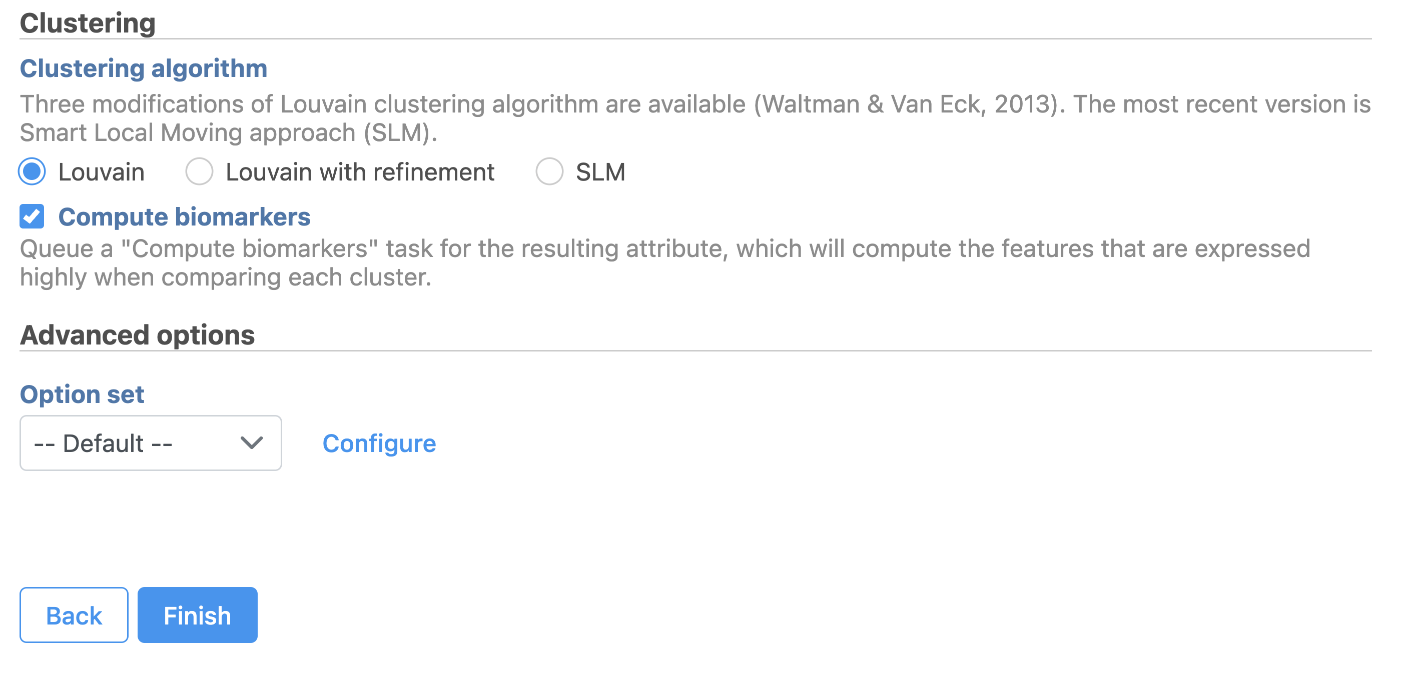
Figure 12. Configure Graph-based clustering in Flow.

A new Graph-based clusters data and a Biomarkers data node will be generated. 

• Double-click the Graph-based clusters node to see the cluster results and statistics (Figure 13)
• Double-click the Biomarkers node to see the computed biomarkers if you have selected this option (Figure 14)

The Graph-based clustering result (Figure 13) lists the Total number of clusters and what proportion of cells fall into each cluster as well as Maximum modularity which is a measurement of the quality of the clustering result where optimal modularity is 1. The Biomarkers report (Figure 14) includes the top features for each graph-based cluster. It displays the top-10 genes that distinguish each cluster from the others. Download at the bottom right of the table can be used to view and save more features. These are calculated using an ANOVA test comparing the cells in each group to all the other cells, filtering to genes that are 1.5 fold upregulated, and sorting by ascending p-value. This ensures that the top-10 genes of each cluster are highly and disproportionately expressed in that cluster. 

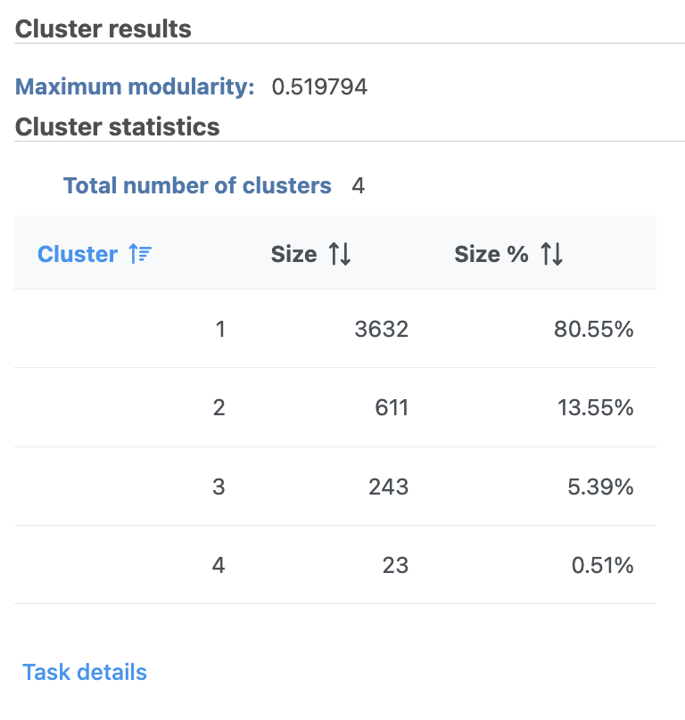
Figure 13. Graph-based clustering results in Flow.

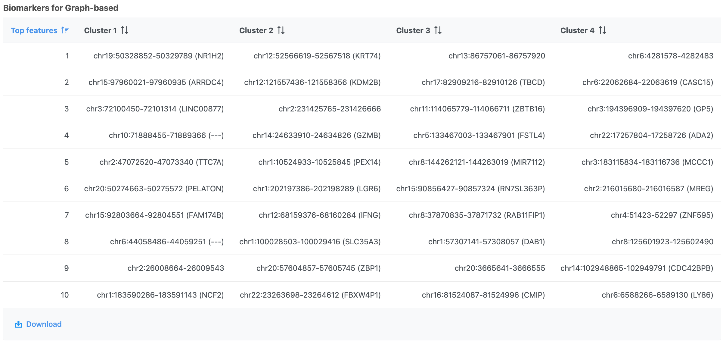
Figure 14. Computer biomarkers results in Flow.

UMAP

Similar to t-SNE, Uniform Manifold Approximation and Projection (UMAP) is a dimensional reduction technique. UMAP aims to preserve the essential high-dimensional structure and present it in a low-dimensional representation. UMAP is particularly useful for visually identifying groups of similar samples or cells in large high-dimensional data sets. 

To run UMAP (Figure 15):

• Click the SVD data node
• Click the Exploratory analysis section of the toolbox
• Click UMAP
• Click Finish to run with default settings

UMAP produces a UMAP task node. Opening the task report launches a scatter plot showing the UMAP results. Each point on the plot is a cell for single cell data. The plot will open in 2D or 3D depending on the user preference.  

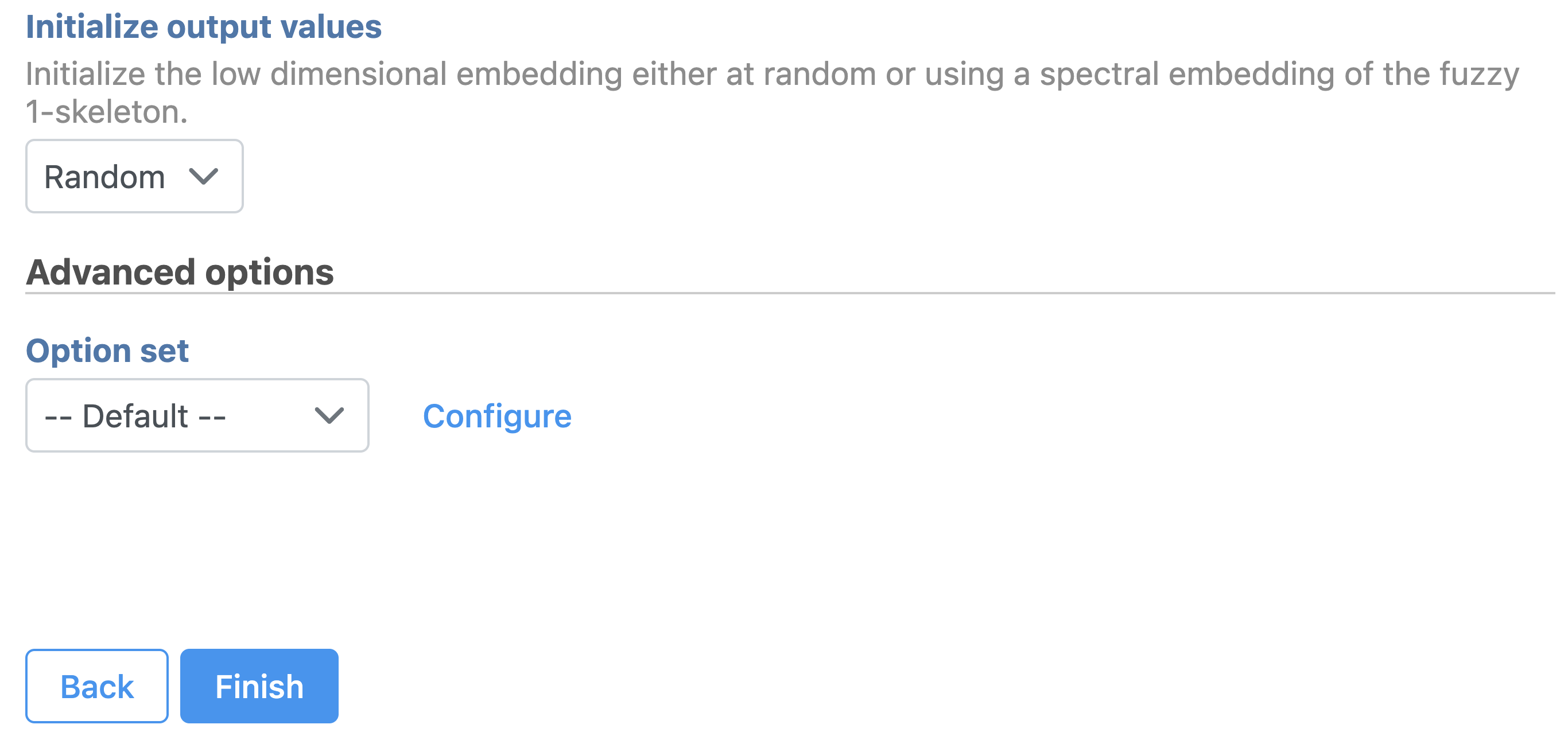
Figure 15. UMAP configuration in Partek Flow.

Promoter sum matrix

The Annotate regions task in Flow labels individual peaks as promoters for a particular gene if the peak falls 1000 bases upstream from a gene's transcription start site, or 100 bases downstream from a gene's transcription start site by default (Figure 9). A promoter sum for a given gene is the number of cut sites per cell that fall within all the peaks labeled as promoters (-1000bp ~ 100bp by default or user defined through Annotate regions) for that gene. Higher promoter sum values indicate higher chromatin accessibility in the promoter region [4]. 

Flow task Promoter sum matrix summarizes each promoter sum and outputs a cell x gene matrix. In the matrix, only genes that have peaks within its promoter region have been included. In Flow Promoter sum matrix can be invoked in the Peak analysis section by clicking the Annotated regions data node (Figure 16).

To run Promoter sum matrix in Flow, 

• Click the Annotated regions data node
• Click the Peak analysis section in the toolbox
• Click Promoter sum matrix

Once the task has been finished, a new data node will be produced where the promoter sum value for each feature can be used to color UMAP/t-SNE and to determine cell type with raw data. We recommend users normalize its output prior to color the UMAP just like the scRNA-seq data.

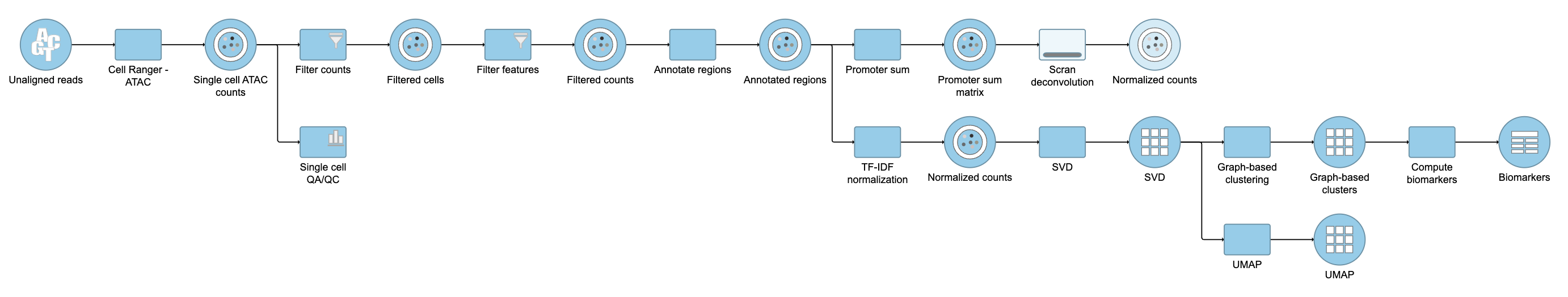
Figure 16. Promoter sum matrix in Flow.

Classifying cells

Double-clicking the UMAP task node will open the task report in the Data Viewer. 

To classify a cell, just select it then click Classify selection in the Classify tool. 

For example, we can classify a cluster of cells expressing high levels of MS4A1 as B cells. 

• Make sure the right data source has been selected. For scATAC-seq data, it shall be the normalized counts of  promoter sum values in most cases (Figure 17) 
• Set Color by in the Style configuration to the normalized counts node
• Type MS4A1 in the search box and select it. Rotate the 3D plot if you need to see this cluster more clearly. 
• Click  to activate Lasso mode
• Draw a lasso around the cluster of MS4A1-expressing cells 
• Click Classify selection under Tools in the left panel
• Type B cells for the Name
• Click Save (Figure 18)

Repeat the above steps to finish the other cell type classifications. To be able to use the classifications in downstream tasks and visualizations, you must first apply them.

• Click Apply classifications
• Name the classification (e.g. Cell type)
• Check the Compute biomarkers if needed
• Click Run to complete the task

Once the classifications have been added  to the project, one can color the UMAP/t-SNE plot by the Classification or compare the differentially expressed genes between different cell types.

Figure 17. Select the data source in Data Viewer.

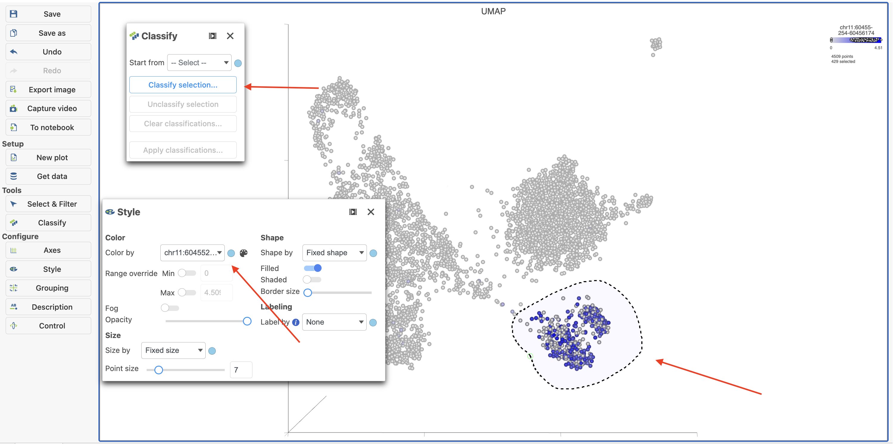
Figure 18. Color cells in UMAP by MS4A1 in Flow.

Differential analysis

To identify genes that distinguish a cell type, one can use the differential analysis tools in Partek Flow.

• Click the TF-IDF normalized counts data node
• Click the Differential analysis section in the toolbox
• Click Hurdle model
• Select the factors and interactions to include in the statistical test (Figure 19). Cell type has been selected here as an example. 

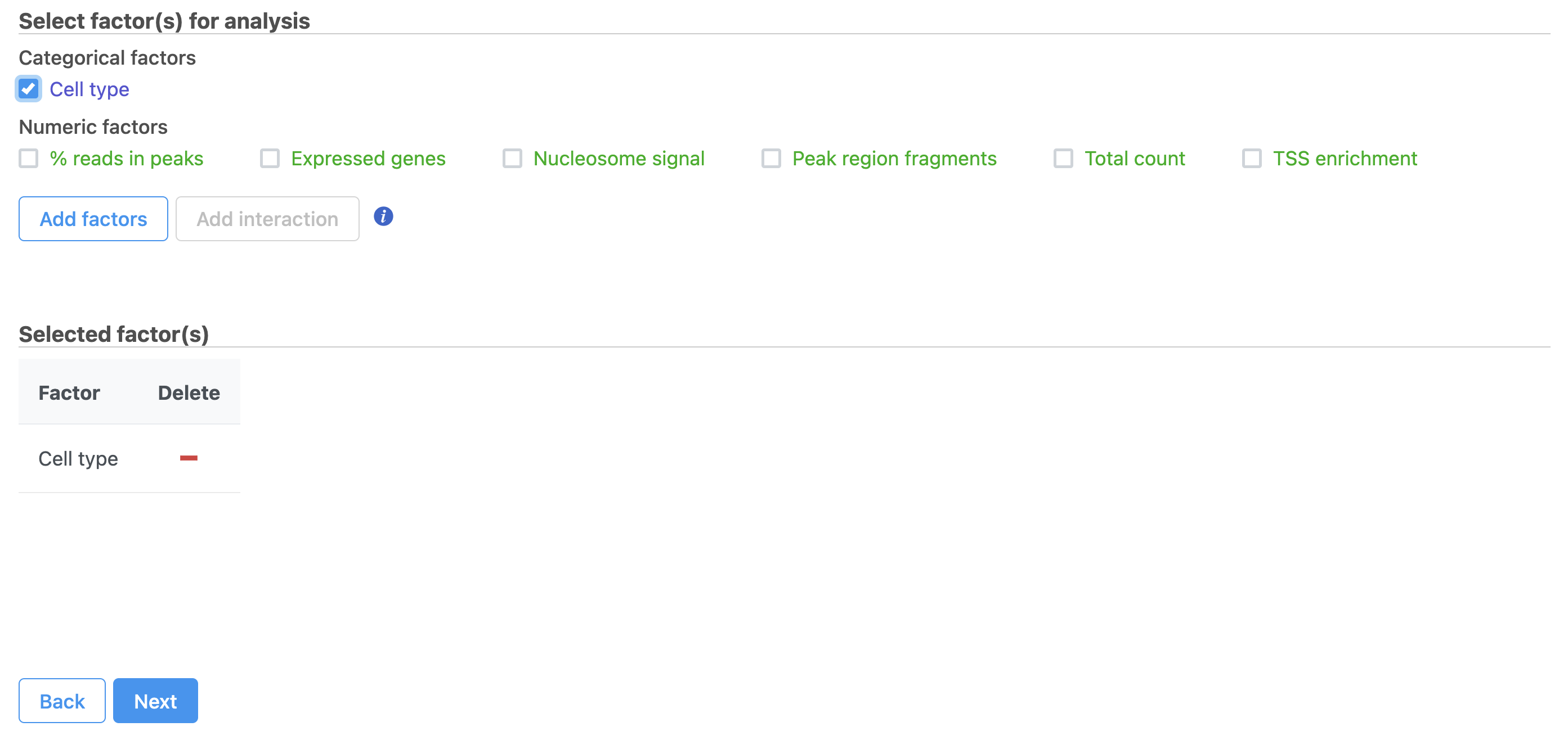
Figure 19. Hurdle model for differential analysis in Flow.

• Click Next 
• Define comparisons between factor or interaction levels (Figure 20)
• Click Add comparison to add the comparison to the Comparisons table. 
• Click Finish to run the statistical test as default

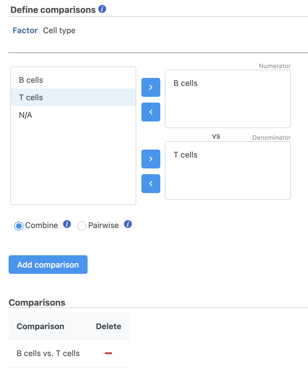
Figure 20. Define comparisons in Hurdle model.

Hurdle model produces a Feature list task node. The results table and options are the same as the GSA task report except the last two columns. The percentage of cells where the feature is detected (value is above the background threshold) in different groups (Pct(group1), Pct(group2)) are calculated and included in the Hurdle model report. 

A filtered Feature list data node can be produced by running the Differential analysis filter in the Hurdle model task report (Figure 21) . 

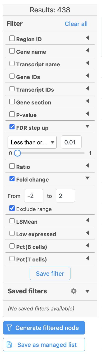
Figure 21. Generate filtered node for differential analysis results in Flow.

Once we have filtered a list of differentially expressed genes, we can visualize these genes by generating a heatmap, or perform the Gene set enrichment analysis and motif detection. 

Pipeline

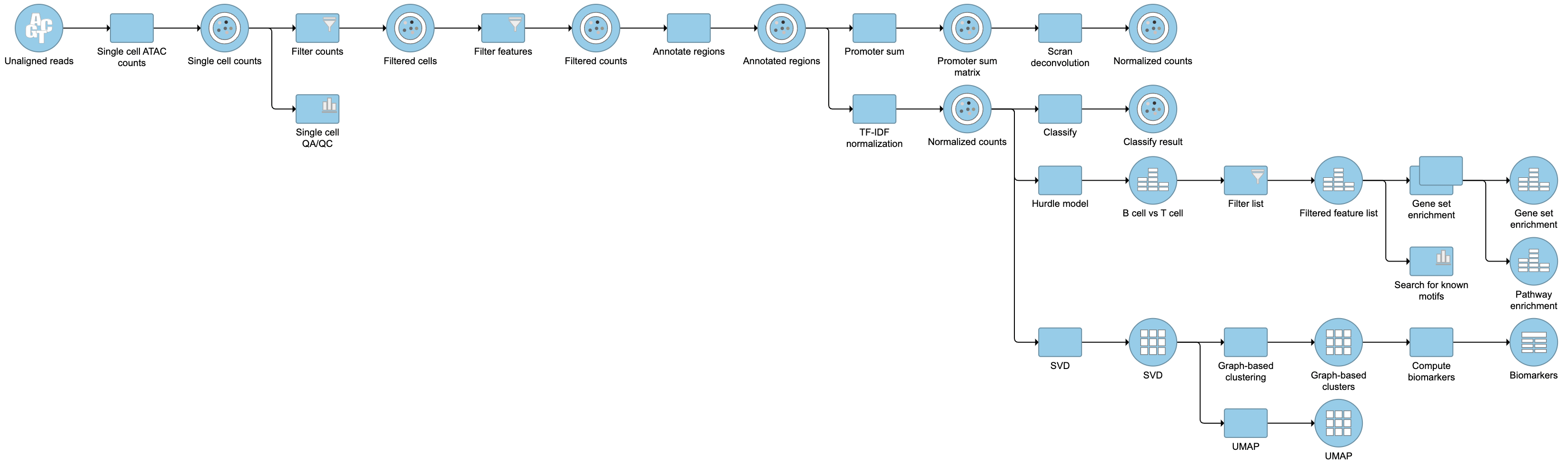
Figure 22. Described pipeline shown in the Analyses tab

For information about automating steps in this analysis workflow, please see our documentation page on Making a Pipeline. 

References

1. https://support.10xgenomics.com/single-cell-atac/software/pipelines/latest/what-is-cell-ranger-atac
2. Cusanovich, D., Reddington, J., Garfield, D. et al. The cis-regulatory dynamics of embryonic development at single-cell resolution. Nature 555, 538–542 (2018). https://doi.org/10.1038/nature25981
3. https://satijalab.org/signac/index.html
4. https://support.10xgenomics.com/single-cell-atac/software/visualization/latest/tutorial-celltypes

Your Rating:

Thanks for voting!

Please Wait

Results:

4

rates