Page History
To detect differential methylation between CpG loci in different experimental groups, we can perform an ANOVA test. For this tutorial, we will perform a simple two-way ANOVA to compare the methylation states of the two experimental groups.
- Select Defect Detect Differential Methylation from the Analysis section of the Illumina BeadArray Methylation workflowSelect 2. State and 3. shRNA treatment
A new child spreadsheet, mvalue, is created when Detect Differential Methylation is selected. M-values are an alternative metric for measuring methylation. β-values can be easily converted to M-values using the following equation: M-value = log2( β / (1 - β)).
An M-value close to 0 for a CpG site indicates a similar intensity between the methylated and unmethylated probes, which means the CpG site is about half-methylated. Positive M-values mean that more molecules are methylated than unmethylated, while negative M-values mean that more molecules are unmethylated than methylated. As discussed by Du and colleagues, the β-value has a more intuitive biological interpretation, but the M-value is more statistically valid for the differential analysis of methylation levels.
Because we are performing differential methylation analysis, Partek Genomics Suite automatically creates an M-values spreadsheet to use for statistical analysis.
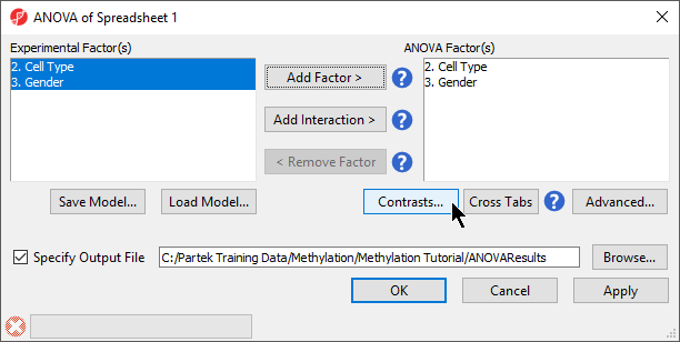
- Select 2. Cell Type and 3. Gender from the Experimental Factor(s) panel by holding the Ctrl key on your keyboard and selecting both itemspanel
- Select Add Factor > to move 2. State andCell Type and 3. shRNA treatment Gender to the ANOVA Factor(s) panel Select Add Interaction > to add the interaction between 2. State and 3. shRNA treatment (Figure 1)
| Numbered figure captions | ||||
|---|---|---|---|---|
| ||||
|
- Select Contrasts...
- Select Yes for Leave Data is already log transformed? set to No
- Leave Report comparisons as set to Difference
For methylation data, fold-change comparisons are not appropriate. Instead, comparisons should be reported as the difference between groups.
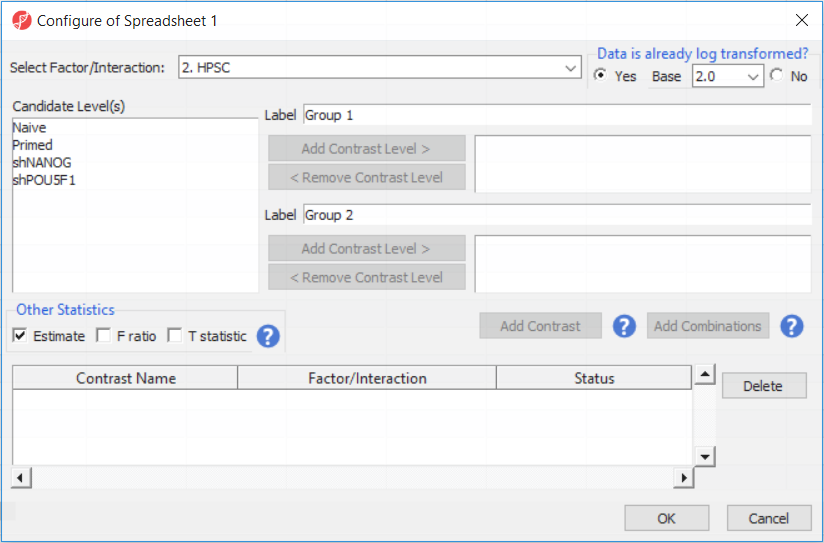
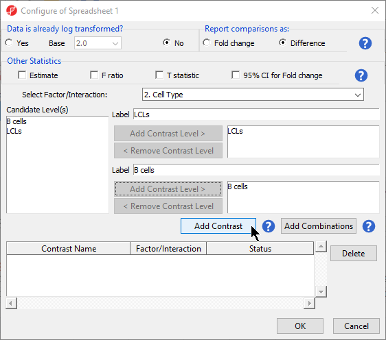
- Select 2. State * 3. shRNA treatment from the Cell Type from the Select Factor/Interaction dropInteraction drop-down menu Select all four options in the Candidate Level(s) panel by selecting each while holding the Ctrl key on your keyboardmenu
- Select LCLs
- Select Add Contrast Level > for Group 1
- Repeat steps to add all four options to Group 2
- Select Add Combination
- Select OK to close the Configuration dialog
- Select OK to close the ANOVA dialog and run the ANOVA
...
- for the upper group
- Select B cells
- Select Add Contrast Level > for the lower group
- Select Add Contrast (Figure 2)
| Numbered figure captions | |
|---|---|
|
...
...
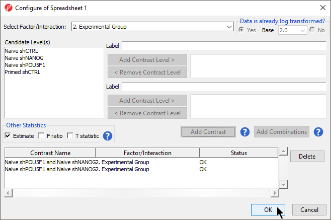
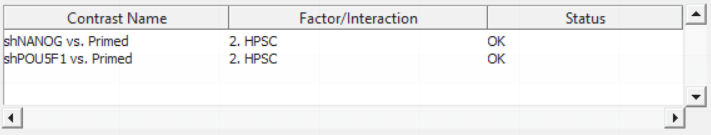
For this exercise, we shall compare primed HPSC with suppression of OCT4 (shPOU5F1) and primed HPSC with suppression of NANOG (shNANOG) with the baseline primed cells. To start with, select the Primed group in the Candidate Level(s) box and push Add Contrast Level > to move the Primed group to Group 2 (lower box). Then Ctrl & select both shPOU5F1 and shNANOG in the Candidate Level(s) box and push Add Contrast Level > to move them to Group 1 (upper box). Then click Add Combinations and confirm that two contrast have been created as seen in Figure 3.
| Numbered figure captions | ||||
|---|---|---|---|---|
| ||||
|
Push OK to confirm the contrast (and close the contrast dialog) and again to start the ANOVA calculation.
...
| |||
|
- Select OK to close the Configuration dialog
The Contrasts... button of the ANOVA dialog now reads Contrasts Included
- Select OK to close the ANOVA dialog and run the ANOVA
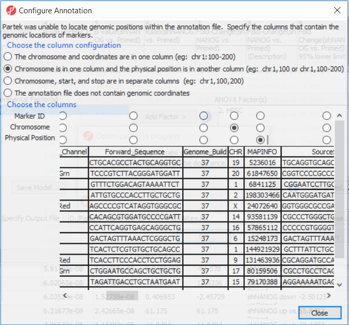
If this is the first time you have analyzed a MethylationEPIC array using the Partek Genomics Suite software, the manifest file may need to be configured. If it needs configuration, the Configure Annotation dialog will appear (Figure 3).
- Select Chromosome is in one column and the physical location is in another column
...
- for Choose the column configuration
- Select Ilmn ID for Marker ID
- Select CHR for Chromosome i
- Select MAPINFO for Physical Position
- Select Close
This enables Partek Genomics Suite to parse out probe annotations from the manifest file.
| Numbered figure captions | ||||
|---|---|---|---|---|
| ||||
|
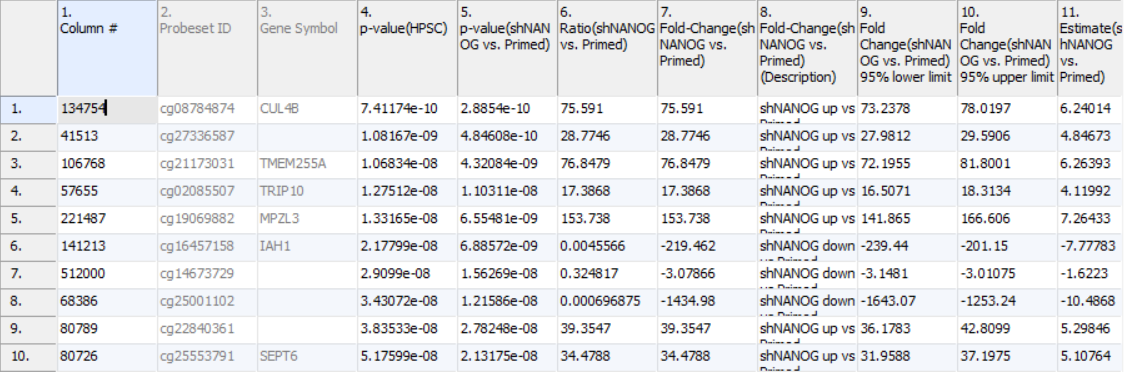
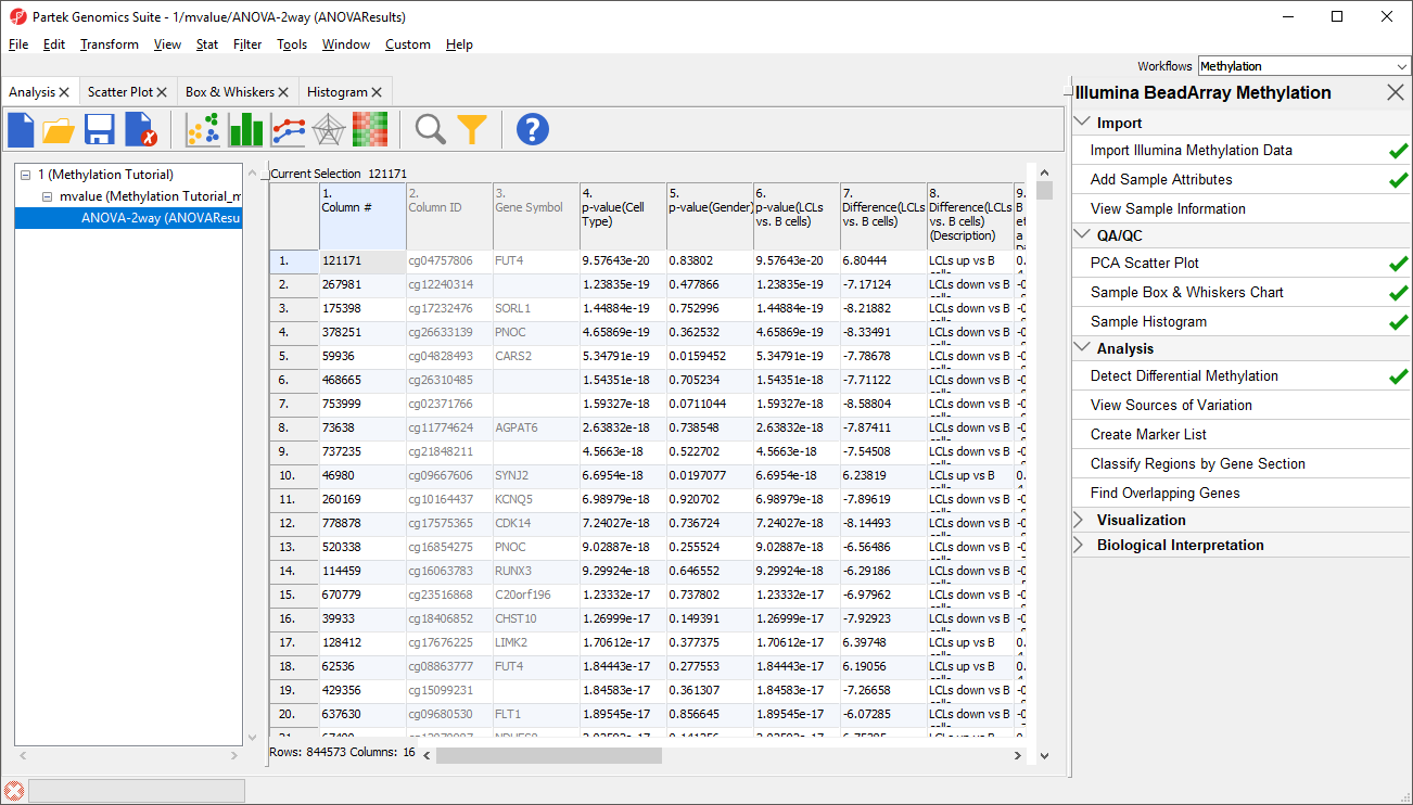
Column 3. Gene Symbol: the gene overlapping the probe as specified in the Illumina manifest file
Column 4. p-value(HPSC): overall p-value for the specified factor (in parenthesis). A low p-value indicates that there is a difference in methylation between the levels of this attribute (i.e. study groups). The contrast p-values should then be used to evaluate individual group comparisons. If more than one factor is included in the model, p-value will be reported for each.
Next, for each contrast included in the model, a block of seven columns will be added, as follows:
Column 5. p-value(shNANOG vs. Primed): p-value for the given contrast (in parenthesis). A low p-value indicates a difference in methylation between the groups included in the contrast (here: shNANOG and Primed).
Column 6. Ratio(shNANOG vs. Primed): ratio of average methylation level in one over the other the other contrasted group (shNANOG and Primed, respectively). Ratio is reported in linear space.
Column 7. Fold Change(shNANOG vs. Primed): fold-change in one over the other contrasted group (shNANOG and Primed, respectively). Fold-change is reported in linear space.
Column 8. Fold Change(shNANOG vs. Primed) (Description): if fold-change > 1, it means hypermethylation in the first group (e.g. shNANOG up vs Primed), if fold-change < -1, it means hypomethylation in the first group (e.g. shNANOG down vs Primed), relative to the second group (Primed). This column enables quick filtering
Columns 9. & 10. Lower and upper (respectively) limits of 95% confidence interval of the fold-change
Column 11. Estimate(shNANOG vs. Primed): difference between means of two groups (i.e. shNANOG and Primed) (this column is optional and depends on the way contrasts were set up)
Columns 12. - 18. correspond to columns 5. - 11.
Columns 19.+ Statistical output
| Numbered figure captions | ||||
|---|---|---|---|---|
| ||||
|
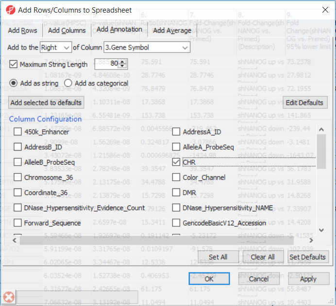
Going forward, analysis of differentially methylated loci typically includes removal of the probes on X and Y chromosomes (to avoid the problems with inactivation of one X chromosome). To annotate the ANOVA spreadsheet with the information required for filtering, right-click on the Gene Symbol column, select Insert Annotation, tick-mark the CHR filed (Figure 6) and push OK. A new column will be appended to the spreadsheet.
| Numbered figure captions | ||||
|---|---|---|---|---|
| ||||
|
To enable filtering right-click on the header of the CHR column > Properties and set the type to categorical (and OK). Now, activate the Interactive Filter tool (![]() ) . If needed use the drop-down list to point to the CHR column. The column chart represents the number of appearances of each chromosome in the spreadsheet (i.e. the number of probes per chromosome). To remove the probes on the X and the Y chromosome left click on the two right-most columns (the pop up balloon will show you the chromosome label) and the columns will be grayed out (Figure 7).
) . If needed use the drop-down list to point to the CHR column. The column chart represents the number of appearances of each chromosome in the spreadsheet (i.e. the number of probes per chromosome). To remove the probes on the X and the Y chromosome left click on the two right-most columns (the pop up balloon will show you the chromosome label) and the columns will be grayed out (Figure 7).
| Numbered figure captions | ||||
|---|---|---|---|---|
| ||||
|

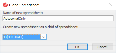
After removal of the probes on the sex chromosomes, let us extract all the autosomal probes to a new spreadsheet. Right click on the ANOVA 1-way spreadsheet > Clone... Set the Name of new spreadsheet to AutosomalOnly and make it a child of the top-level spreadsheet (EPIC iDAT) (Figure 8). Push OK. The newly created autosomalonly spreadsheet will be a new starting point for all the downstream steps.
| Numbered figure captions | ||||
|---|---|---|---|---|
| ||||
|
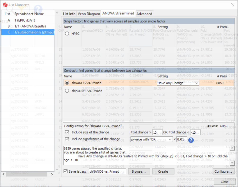
To come up with a list of differentially methylated loci, proceed to the workflow and select Create Marker List. That will open the List Manager functionality and you will be on the ANOVA Streamlined tab. Factors in the model are listed in the top section, contrasts specified in the model are in the middle, while the filter settings are at the bottom.
Select shNANOG vs Primed contrast to see the current filter configuration. By default, both fold-change and p-value with false discovery rate (FDR) correction are applied, with the number of CpG loci passing the filter given as # Pass. For this tutorial, set the fold-change to > 10 and < -10, and reduce the p-value with FDR down to 0.01 (Figure 9). Then push the Create button to save the list of significant loci under the default name (shNANOG vs. Primed). Repeat the procedure for the shPOU5F1 vs Primed, using the same cut offs.
| Numbered figure captions | ||||
|---|---|---|---|---|
| ||||
|
|
| Page Turner | ||
|---|---|---|
|
| Additional assistance |
|---|
|
| Rate Macro | ||
|---|---|---|
|
Overview
Content Tools