Page History
Principal components (PC) analysis (PCA) is an exploratory technique that is used to describe the structure of high dimensional data by reducing its dimensionality. It is a linear transformation that converts n original variables (typically: genes or transcripts) into n new variables, which are called PCs, they have three important properties:
- PCs are ordered by the amount of variance explained
- PCs are uncorrelated
- PCs explain all variation in the data
PCA is a principal axis rotation of the original variables that preserves the variation in the data. Therefore, the total variance of the original variables is equal to the total variance of the PCs.
If read quantification (i.e. mapping to a transcript model) was performed by Partek® E/M algorithm, PCA can be invoked on a quantification output data node (Gene counts or Transcript counts) or, after normalization, on a Normalized counts data node. Select a node on the canvas and then PCA in the Exploratory analysis section of the context sensitive menu.
There are two options for features contribute (Figure 1):
equally: all the features are standardized to mean of 0 and standard deviation of 1 . This option will give all the features equal weight in the analysis, this is the default option for e.g bulk RNA-seq data.
by variance: the analysis will give more emphasis to the features with higher variances. This is the default option for e.g. single cell RNA-seq data
If the input data node is in linear scale, you can perform log transformation on PCA calculation.
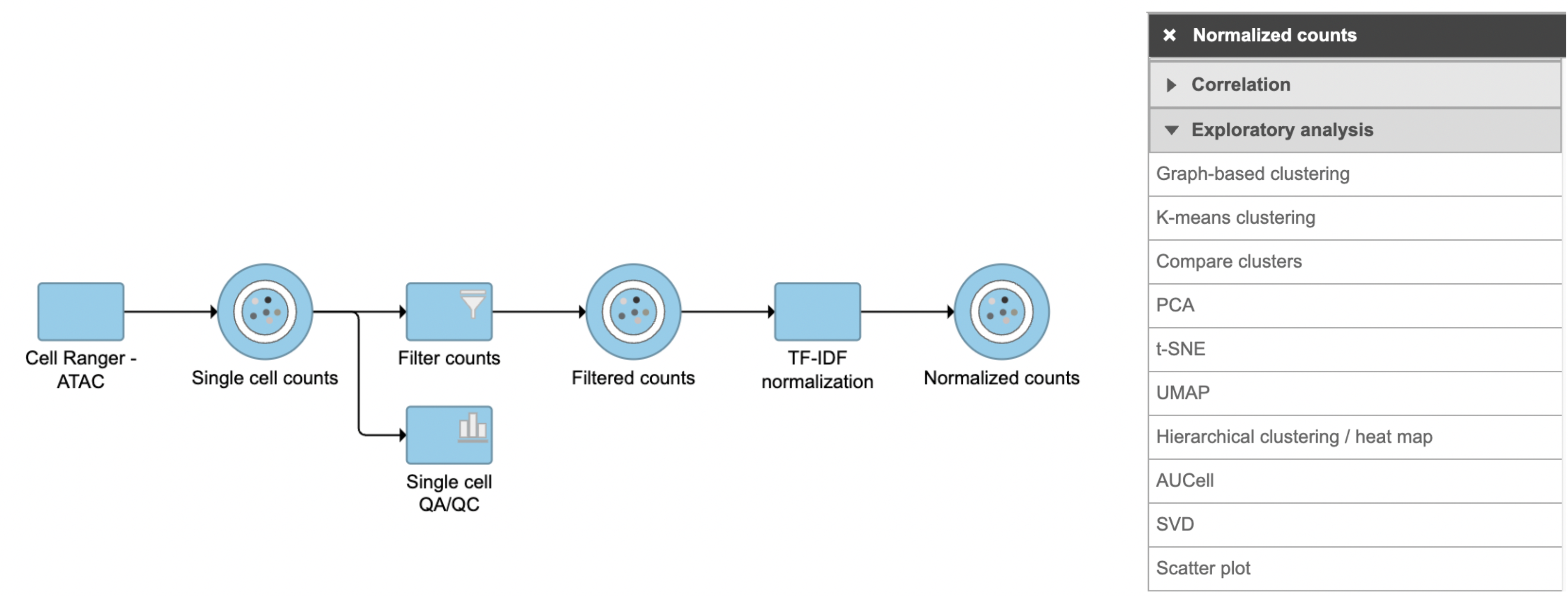
To analyze scATAC-seq data, Partek Flow introduced a new technique - LSI (latent semantic indexing )[1]. LSI combines steps of frequency-inverse document frequency (TF-IDF) normalization followed by singular value decomposition (SVD). This returns a reduced dimension representation of a matrix. Although SVD and Principal components analysis (PCA) are two different techniques, the SVD has a close connection to PCA. Because PCA is simply an application of the SVD. For users who are more familiar with scRNA-seq, you can think of SVD as analogous to the output of PCA. And similarly, the statistical interpretation of singular values is in the form of variance in the data explained by the various components. The singular values produced by the SVD are in order from largest to smallest and when squared are proportional the amount of variance explained by a given singular vector.
SVD task in Flow can be invoked in Exploratory analysis section by clicking any single cell counts data node (Figure 1). We recommend running SVD on the normalized data, particularly the TF-IDF normalized counts for scATAC-seq analysis.
| Numbered figure captions | ||||
|---|---|---|---|---|
| ||||
|

The PCA task creates a new task node, and to open it and see the result, do one of the following: select the PCA task node, proceed to the context sensitive menu and go to the Task result; or double-click on the PCA task node. The report containing eigenvalues, PC projections, component loadings, and mapping error information for the first three PCs.
When open PCA node in Data viewer, by default, it is 3D scatterplot (Figure 2), each dot on the plot represents an observation, while the first three PCs are shown on the X-, Y-, and Z-axis respectively, with the information content of an individual PC is in the parenthesis.
...
|
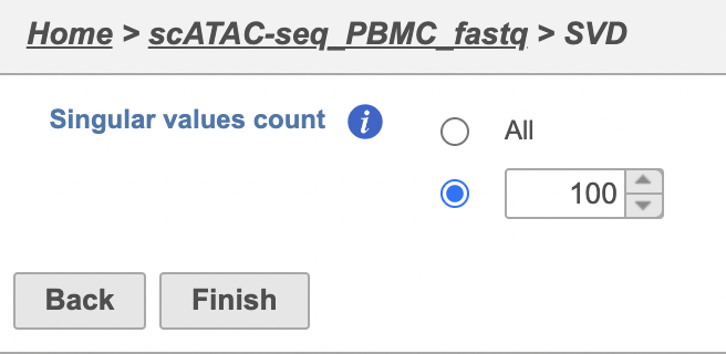
To run SVD task,
- Click a single cell counts data node
- Click the Exploratory analysis section in the toolbox
- Click SVD
The GUI is simple and easy to understand. The SVD dialog is only asking to select the number of singular values to compute (Figure 2). By default 100 singular values will be computed if users don't want to compute all of them. However, the number could be adjusted manually or typed in directly. Simply click the Finish button if you want to run the task as default.
| Numbered figure captions | ||||
|---|---|---|---|---|
| ||||
|

To rotate the plot left click & drag. To zoom in or out, use the mouse wheel. Click and drag the legend can move the legend to different location on the viewer.
Detailed configuration on PCA plot can be found by clicking Help>How-to videos>Data viewer section.
...
| |||
|
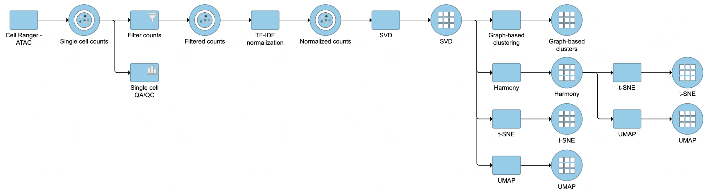
The task report for SVD is similar to PCA. Its output will be used for downstream analysis and visualization, including Harmony (Figure 3).
| Numbered figure captions | ||||
|---|---|---|---|---|
| ||||
|

When choose Scree plot icon ![]() , it will plot a 2D viewer, X-axis represents PCs, Y-axis represents eigenvalues (Figure 4)
, it will plot a 2D viewer, X-axis represents PCs, Y-axis represents eigenvalues (Figure 4)
| Numbered figure captions | ||||
|---|---|---|---|---|
| ||||
|

When mouse over on a point on the line, it will display detailed information of the PC. The scree plot shows how much variation each PC represents, so it is often used to determine the number of principal components to keep for downstream analysis (e.g. tSNE, UMAP, graph-base clustering). The "elbow" point of the graph where the eigenvalues seem to level off should be considered as a cutoff point for downstream analysis.
PCA data node can also be draw as tables, when choose Table icon (![]() ), it will display the component loadings matrix in the viewer (Figure 5)
), it will display the component loadings matrix in the viewer (Figure 5)
| Numbered figure captions | ||||
|---|---|---|---|---|
| ||||
|

In the table, each row is a feature, the column represent PCs, the value is the correlation coefficient. The table can be downloaded as text file. In the configuration panel, the data table drop-down list in the content section, there is PCA projects option, change to this option to display the projection table (Figure 6).
| Numbered figure captions | ||||
|---|---|---|---|---|
| ||||
|

...
| |
|
References
- Cusanovich, D., Reddington, J., Garfield, D. et al. The cis-regulatory dynamics of embryonic development at single-cell resolution. Nature 555, 538–542 (2018). https://doi.org/10.1038/nature25981
Additional Assistance
If you need additional assistance, please visit our support page to submit a help ticket or find phone numbers for regional support.
Overview
Content Tools