Page History
When the reads are aligned to a genome reference, e.g. hg38, the quantification is performed on transcriptome, you need to provide the annotation model file of the transcriptome.
Quantification dialog
If the alignment was generated in Partek® Flow®, the genome assembly will be displayed as text on the top of the page (Figure 1), you do not have the option to change the reference.
| Numbered figure captions | ||||
|---|---|---|---|---|
| ||||
|

If the bam file is imported, you need to select the assembly with which the reads were aligned to, and which annotation model file you will use to quantify from the drop-down menus (Figure 2).
| Numbered figure captions | ||||
|---|---|---|---|---|
| ||||
|

In the Quantification options section, when the Strict paired-end compatibility check button is selected, paired end reads will be considered compatible with a transcript only if both ends are compatible with the transcript. If it is not selected, reads with only one end have alignment that is compatible with the transcript will also be counted for the transcript .
If the Require junction reads to match introns check button is selected, only junction reads that overlap with exonic regions and match the skipped bases of an intron in the transcript will be included in the calculation. Otherwise, as long as the reads overlap within the exonic region, they will be counted. Detailed information about read compatibility can be found in the Understanding Reads tutorial.
Some library preparations reverse transcribe the mRNA into double stranded cDNA, thus losing strand information. In this case, the total transcript count will include all the reads that map to a transcript location. Others will preserve the strand information of the original transcript by only synthesizing the first strand cDNA. Thus, only the reads that have sense compatibility with the transcripts will be included in the calculation. We recommend verifying with the data source how the NGS library was prepared to ensure correct option selection.
In the options, forward means the strand of the read must be the same as the strand of the transcript while reverse means the read must be the complementary strand to the transcript (Figure 3). The options in the drop-down list will be different for paired-end and single-end data. For paired-end reads, the dash separates first- and second-in-pair, determined by the flag information of the read in the BAM file. Briefly, the paired-end Strand specificity options are:
- No: Reads will be included in the calculation as long as they map to exonic regions, regardless of the direction
- Auto-detect: The first 200,000 reads will be used to examine the strand compatibility with the transcripts. Two percentages are calculated: (1) the percentage of reads whose first-in-pair is the same strand as the transcript and second-in-pair is the opposite strand to transcript, (2) the percentage of reads whose first-in-pair is the opposite strand to transcript and second-in-pair is the same strand as the transcript. If the 1st percentage is higher than 75%, the Forward-Reverse option will be used. If the 2nd percentage is higher than 75%, the Reverse-Forward option will be used. If neither of the percentages exceed 75%, No option will be used
- Forward - Reverse: this option is equivalent to the --fr-secondstrand option in Cufflinks [1]. First-in-pair is the same strand as the transcript, second-in-pair is the opposite strand to the transcript
- Reverse - Forward: this option is equivalent to --fr-firststrand option in Cufflinks. First-in-pair is the opposite strand to the transcript, second-in-pair is the same strand as the transcript. The Illumina TruSeq Stranded library prep kit is an example of this configuration
- Forward - Forward: Both ends of the read are matching the strand of the transcript. Generally colorspace data generated from SOLiD technology would follow this format
The single-end Strand specificity options are:
- No: same as for paired-end reads
- Auto-detect: same as for paired-end reads. All single-end reads are treated as first-in-pair reads
- Forward: this option is equivalent to the --fr-secondstrand option in Cufflinks. The single-end reads are the same strand as the transcript
- Reverse: this option is equivalent to --fr-firststrand option in Cufflinks. The single-end reads are the opposite strand to the transcript. The Illumina TruSeq Stranded library prep kit is an example of this configuration
| Numbered figure captions | ||||
|---|---|---|---|---|
| ||||
|

Minimum read overlap with feature can be specified in percentage of read length or number of bases. By default, a read has to be 100% within a feature. You can allow some overhanging bases outside the exonic region by modifying these parameters.
Min reads optioin is a filter, by default only the features whose sum of the reads across all samples that are greater than or equal to 10 will be reported. To report all the features in the annotation file, set the value to 0.
If the Report unexplained regions check button is selected, an additional report will be generated on the reads that are considered not compatible with any transcripts in the annotation provided. Based on the Min reads for unexplained region cutoff, the adjacent regions that meet the criteria are combined and region start and stop information will be reported.
In the annotation file, there might be multiple features in the same location, or one read might have multiple alignments, so the read count of a feature might not be an integer. Our white paper on the Partek E/M algorithm has more details on Partek’s implementation the E/M algorithm initially described by Xing et al. [1]
In ChIP-seq or ATAC-seq analysis, a major challenge after detecting enriched regions or peaks is to compare samples and identify differentially enriched regions. In order to compare samples, a common set of regions must be identified and the number of reads mapping to each region quantified. The Quantify regions task addresses this challenge by generating a union set of unique regions and reporting the number of reads from each sample mapping to each region.
To run Quantify regions:
- Click a Peaks data node
- Click the Quantification section in the toolbox
- Click Quantify regions
Quantify regions method
The Quantify regions task takes MACS2 output, a Peaks or Annotated Peaks data node, as its input. In a typical ATAC-Seq or ChIP-Seq analysis, MACS2 is configured to output a set of enriched regions or peaks for each experimental sample or group individually. Quantify regions takes these sets of regions and merges them into a union set of unique regions that it saves as a .bed file. To combine the region sets, overlapping regions between samples/groups are merged. Where overlap ends, a break point is created and a new region defined. All non-overlapping or unique regions from each sample/group are also included.
For example, consider an experiment where MACS2 detected enriched regions for two samples, Sample A and Sample B. In Sample A, a region is detected on chromosome 1 from 100bp to 300bp, chr1:100-300. In Sample B, a region is detected at chr1:160-360. The Quantify regions task will give the following union set of unique regions for these partially overlapping regions:
chr1:100-160 (region detected in Sample A only)
chr1:160-300 (region detected in both Sample A and Sample B)
chr1:300-360 (region detected in Sample B only)
After generating a .bed file with the union set of unique regions, Quantify regions performs quantification using the same algorithm as Quantify to annotation model (Partek E/M) with the .bed file as the annotation model.
Configuring Quantify regions
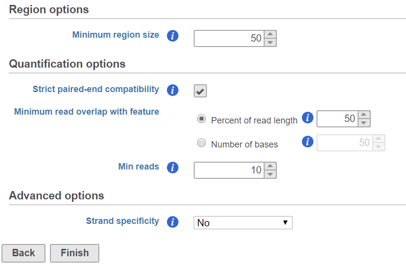
The Quantify regions dialog includes configuration options for generating the union set of unique regions and quantifying reads to the regions (Figure 1).
When regions from multiple samples are combined, a small offset in position between enriched regions in different samples can result in many very short unique regions in the union set. The Minimum region size option lets you filter out these very short regions. If a region is smaller than the specified cutoff, the region is excluded. By default, this is set to 50bp, but may need to be adjusted depending on the size of regions you expect to see in your assay.
Quantification options are the same as in the Quantify to annotation model (Partek E/M)
...
Depending on the annotation file, the output could be one or two data nodes. If the annotation file only contains one level of information, e.g. miRNA annotation file, you will only get one output data node. On the other hand, if the annotation file contains gene level and transcript level information, such as those from the Ensembl database, both gene and transcript level data nodes will be generated. If two nodes are generated, the Task report will also contain two tabs, reporting quantification results from each node. Each report has two tables. The first one is a summary table displaying the coverage information for each sample quantified against the specified transcriptome annotation (Figure 4). dialog. The Percent of read length is set to 50% by default to account for small offsets in position between enriched regions in different samples.
| Numbered figure captions | ||||
|---|---|---|---|---|
| ||||
|

The second table contains feature distribution information on each sample and across all the samples, number of features in the annotation model is displayed on the table title (Figure 5).
| Numbered figure captions | ||||
|---|---|---|---|---|
| ||||
|

The bar chart displaying the distribution of raw read counts is helpful in assessing the expression level distribution within each sample. The X-axis is the read count range, Y axis is the number of features within the range, each bar is a sample. Hovering your mouse over the bar displays the following information (Figure 6):
- Sample name
- Range of read counts, “[ “represent inclusive, “)” represent exclusive, e.g. [0,0] means 0 read counts; (0,10] means the range is greater than 0 count but less than and equal to 10 counts.
- Number of features within the read count range
- Percentage of the features within the read count range
| Numbered figure captions | ||||
|---|---|---|---|---|
| ||||
|

The coverage breakdown bar chart is a graphical representation of the reads summary table for each sample (Figure 7)
| Numbered figure captions | ||||
|---|---|---|---|---|
| ||||
|

...
| |||
|
Quantify regions output
Quantify regions generates a counts data node with the number of counts in each region for each sample. This data node can be annotated with gene information using the Annotate regions task and analyzed using tasks that take counts data as input, such as normalization, PCA, and ANOVA. For ChIP-Seq experiments with input control samples, the Normalize to baseline task can be used prior to downstream analysis.
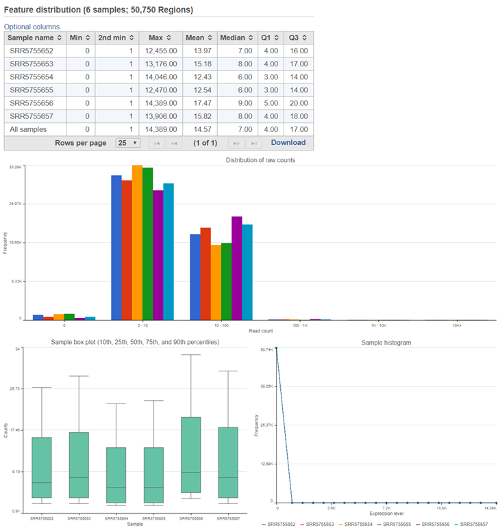
Similar to the Quantify to annotation model (Partek E/M) task report, the Quantify regions task report includes feature distribution information including a descriptive stats table, a distribution bar chart, a sample box plot, and sample histogram (Figure 2).
- Sample name
- Range of read counts, “[ “represent inclusive, “)” represent exclusive
- Number of features within the read count range in the sample
| Numbered figure captions | ||||
|---|---|---|---|---|
| ||||
|

The box whisker and sample histogram plots are helpful for understanding the expression level distribution across samples. This may indicate that normalization between samples might be needed prior to downstream analysis. Note that all four visualizations are disabled for results with more than 30 samples.
The output data node contains raw reads of each sample on each feature (gene or transcript or miRNA etc.depends on the annotation used). When click on a output data node, e.g. transcript counts data node, choose Download data on the context sensitive menu on the right, the raw reads of transcripts can be downloaded in two different format (Figure 10):
Partek Genomics Suite project format: it is a zip file, do not manually unzip it, you can choose File>Import>Zipped project in Partek Genomics Suite to import the zip file into PGS.
Text file format: it is a .txt file, you can open the text file in any text editor or Microsoft Excel, each row is a transcript, each column is a sample.
| Numbered figure captions | ||||
|---|---|---|---|---|
| ||||
|

| Numbered figure captions | ||||
|---|---|---|---|---|
| ||||
|

...
| |||
|
To download the .bed file with the union set of unique regions, click the Quantify regions task node, click Task details, click the regions.bed file in the Output files section, and click Download.
References
- Xing Y, Yu T, Wu YN, Roy M, Kim J, Lee C. An expectation-maximization algorithm for probabilistic reconstructions of full-length isoforms from splice graphs. Nucleic Acids Res. 2006; 34(10):3150-60.
...
Overview
Content Tools