Page History

...

Create a new project to upload your data. Ensure that you have transferred the filtered contig_annotations.csv file(s)² for each sample from either the cellranger vdj⁷ or cellranger multi⁸pipeline to the server, as well as the filtered feature barcode matrices in H5⁴ or MEX⁵ format from the cellranger multi pipeline for each sample if you have matching gene expression data.
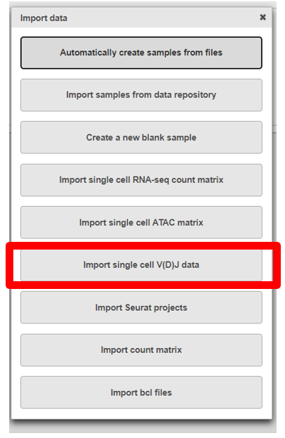
Click Import, then select Import single cell V(D)J data

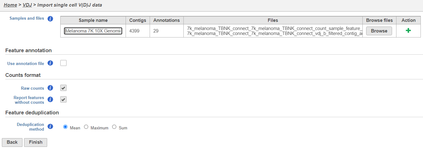
Upload either the filtered contig_annotations.csv file alone or, if you have matching gene expression, with the filtered count matrix per sample and give each sample a name. To add a sample use the the Action. In the example below using default settings, there is one sample with two files, one for V(D)J and one for gene expression. Click Finish.

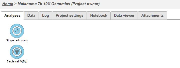
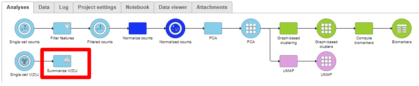
This results in two starting nodes, one for single cell counts and one for single cell V(D)J as shown below. Note that once subsequent tasks are performed on a node, no more data can be imported into this project. The single cell counts node can be processed as usual; for help related to this please see the tutorial for Analyzing Single Cell RNA-Seq Data.

Analyzing the Single cell V(D)J node

...

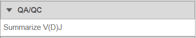
Under QA/QC tasks is the Summarize V(D)J task which will summarize the V(D)J contents by Sample name, # Cells, Barcode count, Clonotypes, Variable genes, Diversity genes, Joining genes, and Constant genes.

Double-click on the completed task to view the contents which can be downloaded.

...

The example below shows the results from the Clonotype Frequency Plot task which is accessed by choosing to perform this task from the Single cell V(D)J node then modified in the data viewer. In this case, the barcode frequency is the number of clonotypes per cell because the barcode usually represents a single cell, so there are two cells which have clonotype5 (purple bar with information from hovering) and clonotype 5 is made of two compositions (a frequency of four for clonotype5 from the V(D)J node) witnessed by the Chain, V gene, D gene, and J gene seen below the bars and by hovering.

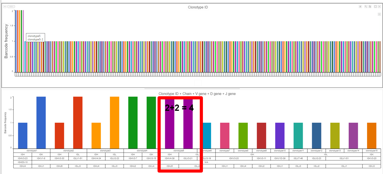
Plotting Clonotype ID frequency, as seen below, for the gene expression node (Cell counts as the top bar chart) and VDJ node (VDJ counts as the bottom bar chart), highlights the difference between the two nodes (where the top plot is the number of cells per clonotype and the bottom plot is the number of V(D)J clonotypes present). Note that Cell Ranger does not always call the barcode as a cell and this can affect these frequencies when making comparisons between cell frequency per clonotype and barcode frequency per clonotype (an example of this would be clonotype1 when comparing the figure above and below).

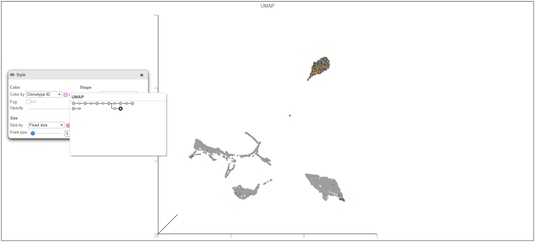
When overlaying the Clonotype ID on plots from the Single cell counts analysis pipeline (such as the UMAP example below), make sure that the Clonotype ID from the Single cell counts node and not the VDJ node is used.

B cell isotypes are defined by Chain and C gene. In the example below, Chain and C gene are plotted by Barcode frequency. On the left, no selection and filtering has been performed. On the plot on the right, the heavy chain has been selected and filtered by in the data. By using select & filter, criteria can be selected and focused on.

In the left plot below, CDR3 abundance is plotted by barcode frequency and colored by Clonotype ID. In the example on the right, the plot is instead colored by Chain and other modifications have been made such as axis ticks and the number of groups per page. Note that the predicted CDR3 amino acid sequence is plotted here, but the predicted CDR3 nucleotide sequence (cdr3_nt) as well as information for other Complementarity-Determining Regions is also available.

Image Added Image Added

In the plot on the left below, barcode frequency for V genes is sorted by frequency in descending order and colored by Chain. The transposed plot on the right shows all of the groups sorted by ascending value and the heavy chain has been excluded. Gene usage plots for the D and J genes can be quickly shown by changing the data dropdown.

Image RemovedImage RemovedImage AddedImage Added