Page History
...
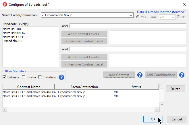
- Select Contrasts...
- Select Yes for Data is already log transformed? because M-values are based on logit transformation
- Select Naive shPOU5F1
- Select Add Contrast Level > for the upper group
- Repeat to add Naive shNANOG to add Naive shNANOG and Primed shCTRL to the upper group
- Select Naive shCTRL shCTRL
- Select Add Contrast Level > for the lower group
- Select Add Contrast
- Repeat steps to create an additional contrast: Naive shPOU5F1 and Naive shNANOG vs. Primed shCTRL
- Select the Estimate box in the Other Statistics section of the Configure dialog (Figure 2)
...
| Numbered figure captions | ||||
|---|---|---|---|---|
| ||||
|
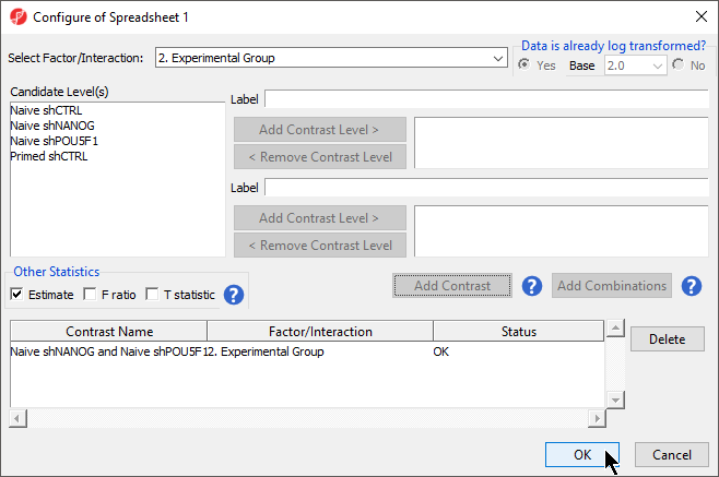
- Select Add Combination
- Select OK to close the Configuration dialog
...
| Numbered figure captions | ||||
|---|---|---|---|---|
| ||||
|
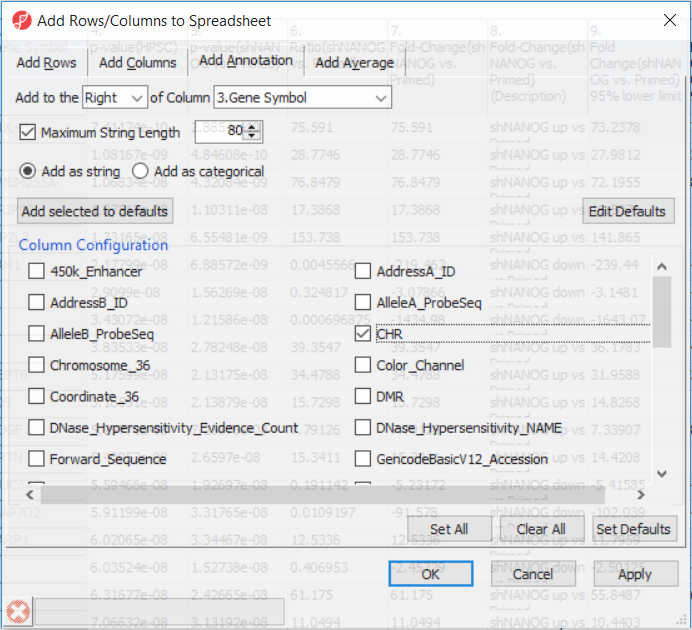
Going forward, analysis of differentially methylated loci typically includes removal of the probes on X and Y chromosomes (to avoid the problems with inactivation of one X chromosome). To annotate the ANOVA spreadsheet with the information required for filtering, right-click on the Gene Symbol column, select Insert Annotation, tick-mark the CHR filed (Figure 6) and push OK. A new column will be appended to the spreadsheet.
| Numbered figure captions | ||||
|---|---|---|---|---|
| ||||
|
To enable filtering right-click on the header of the CHR column > Properties and set the type to categorical (and OK). Now, activate the Interactive Filter tool (![]() ) . If needed use the drop-down list to point to the CHR column. The column chart represents the number of appearances of each chromosome in the spreadsheet (i.e. the number of probes per chromosome). To remove the probes on the X and the Y chromosome left click on the two right-most columns (the pop up balloon will show you the chromosome label) and the columns will be grayed out (Figure 7).
) . If needed use the drop-down list to point to the CHR column. The column chart represents the number of appearances of each chromosome in the spreadsheet (i.e. the number of probes per chromosome). To remove the probes on the X and the Y chromosome left click on the two right-most columns (the pop up balloon will show you the chromosome label) and the columns will be grayed out (Figure 7).
| Numbered figure captions | ||||
|---|---|---|---|---|
| ||||
|

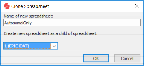
After removal of the probes on the sex chromosomes, let us extract all the autosomal probes to a new spreadsheet. Right click on the ANOVA 1-way spreadsheet > Clone... Set the Name of new spreadsheet to AutosomalOnly and make it a child of the top-level spreadsheet (EPIC iDAT) (Figure 8). Push OK. The newly created autosomalonly spreadsheet will be a new starting point for all the downstream steps.
| Numbered figure captions | ||||
|---|---|---|---|---|
| ||||
|
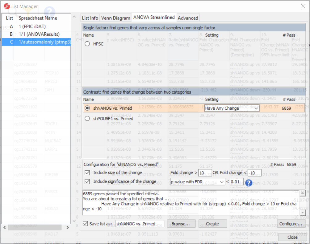
To come up with a list of differentially methylated loci, proceed to the workflow and select Create Marker List. That will open the List Manager functionality and you will be on the ANOVA Streamlined tab. Factors in the model are listed in the top section, contrasts specified in the model are in the middle, while the filter settings are at the bottom.
Select shNANOG vs Primed contrast to see the current filter configuration. By default, both fold-change and p-value with false discovery rate (FDR) correction are applied, with the number of CpG loci passing the filter given as # Pass. For this tutorial, set the fold-change to > 10 and < -10, and reduce the p-value with FDR down to 0.01 (Figure 9). Then push the Create button to save the list of significant loci under the default name (shNANOG vs. Primed). Repeat the procedure for the shPOU5F1 vs Primed, using the same cut offs.
| Numbered figure captions | ||||
|---|---|---|---|---|
| ||||
|
| Page Turner | ||
|---|---|---|
|
| Additional assistance |
|---|
|
| Rate Macro | ||
|---|---|---|
|
Overview
Content Tools