Introducing Survival Analysis

Survival analysis is a branch of statistics that deals with modeling of time-to-event. In the context of “survival,” the most common event studied is death; however, any other important biological event could be analyzed in a similar fashion (e.g., spreading of the primary tumor or occurrence/relapse of disease). Survival analysis tries to answer questions such as: What is the proportion of a population who will survive past a certain time (i.e., what is the 5-year survival rate)? What is the rate at which the event occurs? Do particular characteristics have an impact on survival rates (e.g., are certain genes associated with survival)? Is the 5-year survival rate improved in patients treated by a new drug? Cox regression and Kaplan-Meier analysis are two techniques which are commonly used to assess survival analysis. 

In survival analysis, the event should be well-defined with two levels and occur at a specific time. Because the primary outcome of the event is typically unfavorable (e.g., death, metastasis, relapse, etc.), the event is called a “hazard.” The hazard ratio is used to assess the likelihood of the event occurring while controlling for other co-predictors (co-variables/co-factors) if added to the model. In other words, the hazard ratio is how rapidly an event is experienced by comparing the hazard between groups. A hazard ratio greater than 1 indicates a shorter time-to-event (increase in the hazard), a hazard ratio less than 1 is associated with a greater time-to-event (reduction in the hazard), and a hazard ratio of 1 indicates no effect on time-to-event. For example, if the hazard ratio is 2 then there is twice a chance of occurrence compared to the other group. In cancer studies, a hazard ratio greater than 1 is considered a bad prognostic factor while a hazard ratio less than 1 is a good prognostic factor. Click here for more information on hazard ratios.

An important aspect of survival analysis is “censored” data. Censored data refers to subjects that have not experienced the event being studied. For example, medical studies often focus on survival of patients after treatment so the survival times are recorded during the study period. At the end of the study period, some patients are dead, some patients are alive, and the status of some patients is unknown because they dropped out of the study. Censored data refers to the latter two groups. The patients who survived until the end of the study or those who dropped out of the study have not experienced the study event "death" and are listed as "censored". 

Cox Regression

Cox regression (Cox proportional-hazards model) tests the effects of factors (predictors) on survival time. Predictors that lower the probability of survival at a given time are called risk factors; predictors that increase the probability of survival at a given time are called protective factors. The Cox proportional-hazards model are similar to a multiple logistic regression that considers time-to-event rather than simply whether an event occurred or not. Cox regression should not be used for a small sample size because the events could accidently concentrate into one of the cohorts which will not produce meaningful results. Click here to read more about hazard ratio estimation in small samples.

Configuring the Cox Regression Dialogue 

• Open the Cox Regression task in the task menu under Statistics for any counts node. 

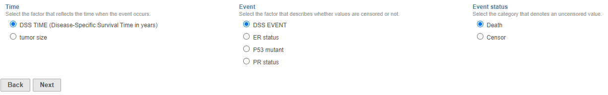
• Next, select the Time, Event, and Event status. Partek Flow will automatically guess factors that might be appropriate for these options. Click Next to proceed with the task. 

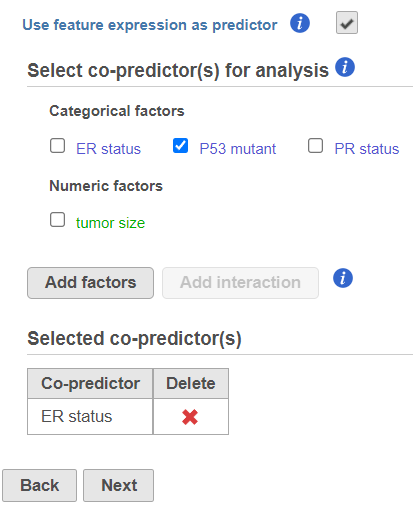
• The predictors (factors or variables) and co-predictors in the model must be defined. Co-predictors are numeric or categorical factors that will be included in the cox regression model. Time-to-event will be performed on features (e.g. genes) by default unless Use feature expression as predictor is unchecked. If unchecked, select a factor and Add factors that is not features to model a different variable. Using the default setting, Use feature expression as predictor, lets the user Add factors to the model that act to explain the relationship for time-to-event (co-predictor) in addition to features. Choose Add interaction to add co-predictors with known dependencies. If factors are added here, they cannot be added as stratification factors. Click Next to proceed with the task. 

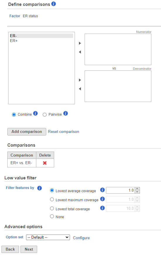
• Next, the user can define comparisons for the co-predictors if they have been added. Configure contrasts by moving factors into the numerator (e.g. experimental factor) or denominator (e.g. control factor / reference), choose Combine or Pairwise, and add the comparison which will be displayed below. Combine all numerator levels and combine all denominator levels in a single comparison or choose Pairwise to split all numerator levels and split all denominator levels into a factorial set of comparisons meaning every numerator will be paired with every denominator. Multiple comparisons from different factors can be added with Add comparison. Low value filter can be used to filter by excluding features; choose a filter or select none. Click Next to proceed with the task. 

• The user can select categorical factors to perform stratification if needed. Stratification is needed because the proportional odds assumption holds only within each stratum, but not across the strata. When stratification factors are included, the proportional hazard assumption will hold for each combination of levels of stratification factor; a separate submodel is estimated for each level combination and the results are aggregated. Click Finish to complete the task. 

• The results of Cox regression analysis provide key information to interpret, including:
  • Hazard ratio (HR): if the HR = 0.5 then half as many patients are experiencing the event compared to the control group, if the HR = 1 the event rates are the same in both groups, and if the HR = 2 then twice as many are experiencing an event compared to the control group. 
  • HR limit: this is the confidence interval of the hazard ratio. 
  • P-value: the lower the p-value, the greater the significance of the observation. 

(e.g. If you have selected both a co-predictor and strata factor then a comparison using the co-predictors and Type III p-value  for the co-predictor will be generated in the Cox regression report.)

Kaplan-Meier Survival Curve 

The Kaplan-Meier task is used for comparing the survival curves among two or more groups of samples. The groups are defined by one or more categorical attributes (factors) specified by the user. Like in the case of Cox Regression, it is possible to use feature expression data, if available. In that case, quantitative feature expression is converted into a feature-specific categorical attribute. Each combination of the attribute levels corresponds to a distinct group. If one selects three factors with 2, 3 and 5 levels, respectively, then the total count of compared groups is 2*3*5 = 30. Therefore, selecting too many factors and/or factors with many levels may not work since the total number of samples may be not enough to fill all of the groups.

To perform Kaplan-Meier survival analysis, at least two pieces of information must be provided for each sample: time-to-event (a numeric factor) and event status (categorical factor with two levels). Time-to-event indicates the time elapsed between the enrollment of a subject in the study and the occurrence of the event. Event status indicates whether the event occurred or the subject was censored (did not experience the event). The survival curve is not straight lines connecting each point, instead a staircase pattern is used. The event status will determine the staircase pattern where each drop in the staircase represents the event occurrence. 

Getting started with the Kaplan-Meier task

The Kaplan-Meier task begins similar to the Cox regression task, then differs when selecting categorical attributes to define the compared groups. 

For each feature (e.g. gene), the expression values are sorted in ascending order and placed into B bins of (roughly) equal size. As a result, a feature-specific categorical attribute with B levels is constructed which can be used by itself or in combination with other categorical attributes. For instance, for B = 2 (Figure 1), we take a given feature and compute its median expression. The samples are separated into two bins, depending on whether the expression in the sample is below or above the median.  if two percentiles are chosen, the bins are automatically labeled "Low" and "High" but the text box can be used to re-label the bins. The bins are feature-specific since this procedure is repeated for each feature separately.

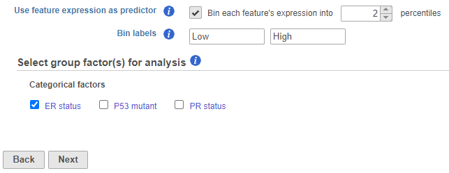
Figure 1. Selecting categorical attributes to define compared groups

For each group, the survival curve (aka survival function) is estimated using Kaplan-Meier estimator [1]. For instance, if one selects ER status which has two levels and we choose two feature expression bins, four survival curves are displayed in the Data Viewer (Figure 2). The Grouping configuration option can be used to split and modify the connections. 

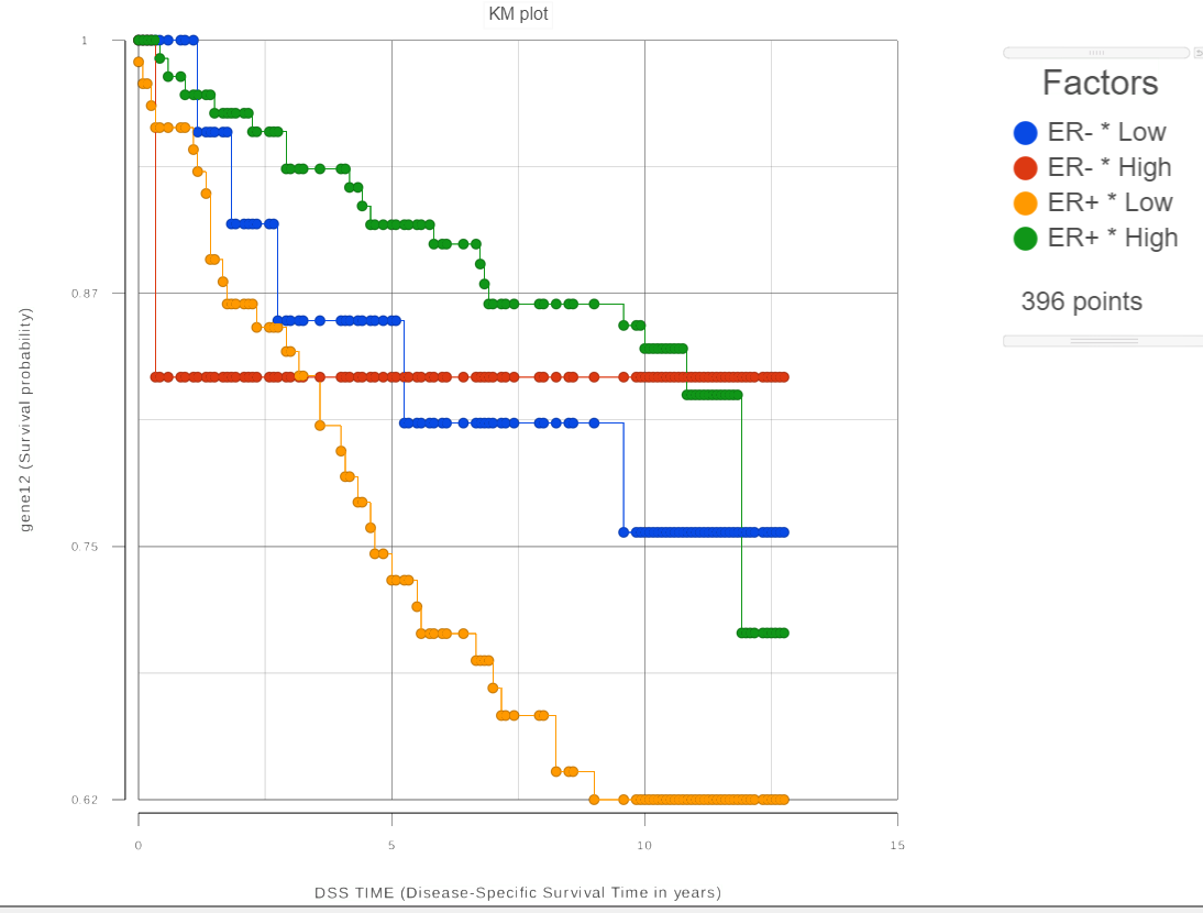
Figure 2. Each of the defined groups produces a survival curve

To see whether the survival curves are statistically different, Kaplan-Meier task runs Log-rank and Wilcoxon (aka Wilcoxon-Gehan) tests. The null hypothesis is that the survival curves do not differ among the groups (the computational details are available in [2]). When feature expression is used, the p-values are also feature specific (Figure 3). Select the step-plot icon under View to visualize the Kaplan-Meier survival curves for each gene. 

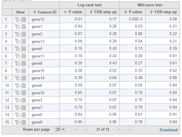
Figure 3. Log-rank and Wilcoxon p-values when feature expression is used

Choosing stratification factors

Like in Cox Regression task, it is possible to choose stratification factor(s), but the purpose and meaning of stratification are not the same as in Cox Regression. Suppose we want to compare the survival among the four groups defined by the two levels of ER status and the two bins of feature expression. We can select the two factors on  “Select group factor(s)” page (Figure 1). In that case, the reported p-values will reflect the statistical difference among the four survival curves that are due to both ER status and the feature expression. Imagine that our primary interest is the effect of feature expression on survival. Although ER status can be important and therefore should be included in the model, we want to know whether the effect of feature expression is significant after the contribution of ER status is taken into account. In other words, the goal is to treat ER status as a nuisance factor and the binned feature expression as a factor of interest.

In qualitative terms, it is possible to obtain an answer if we group the survival curves by the level of ER status. This can be achieved in the Data Viewer by choosing Grouping > Split by under Configure (Figure 4). That makes it easy to compare the survival curves that have the same level of ER status and avoid the comparison of curves across different levels of ER status.

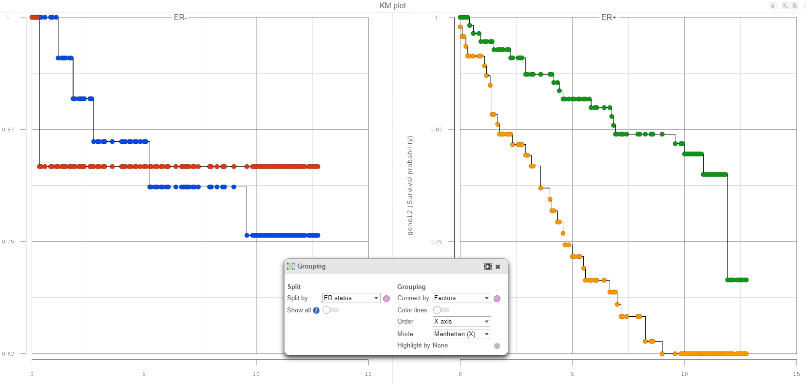
Figure 4. Grouping of survival curves by the level of a specified factor

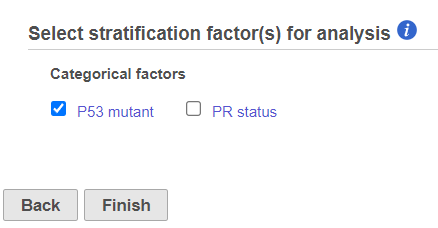
If in Figure 4, we see one or more subplots where the survival curves differ a lot, that is evidence that the feature expression affects the survival even after adjusting for the contribution of ER status. To obtain an answer in terms of adjusted Log-rank and Wilcoxon p-values, one should deselect ER status as a “group factor” (Figure 1) and mark it as a stratification factor instead (Figure 5). The computation of stratification adjusted p-values is elaborated in [2].

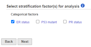
Figure 5. Selecting one or more stratification factors

Suppose when the feature expression and ER status are selected as “group factors” (Figure 1), Log-rank p-value is 0.001, and when ER status is marked as stratification factor, the p-value becomes 0.70. This means that ER status is very useful for explaining the difference in survival while the feature factor is of no use if ER status is already in the model. In other words, the marginal contribution of the binned expression factor is low. 

If more than two attributes are present, it is possible to measure the marginal contribution of any single factor in a similar manner: the attribute of interest should be selected as “group factor” (Figure 1) and the other attributes should be marked as stratification factors (Figure 5). There is no limit on the count of factors that can be selected as “group” or stratification, except that all of the selected factors are involved in defining the groups and the groups should contain enough samples (at least, be non-empty) for the results to be reliable. 

Troubleshooting

If the task fails (no report is produced), please follow the directions in Reporting a problem.

If the task report is produced, but the results are missing for some features, it may be possible to fix the issue by following the directions in the Differential Analysis Troubleshooting section.

References

[1] Kaplan-Meier (product limit) estimator: https://en.wikipedia.org/wiki/Kaplan%E2%80%93Meier_estimator

[2] Klein, Moeschberger (1997), Survival Analysis: Techniques for Censored and Truncated Data. ISBN-13: 978-0387948294

Your Rating:

Thanks for voting!

Please Wait

Results:

6

rates