Selecting a node with unaligned reads (either Unaligned reads or Trimmed reads) shows the QA/QC section in the context sensitive menu, with two options (Figure 1). To assess the quality of your raw reads, use Pre-alignment QA/QC.
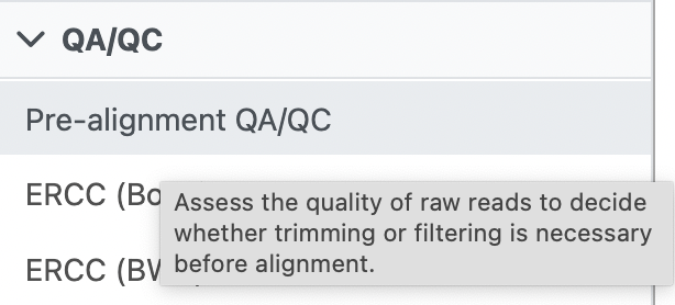
Figure 1. QA/QC options on unaligned reads
Pre-alignment QA/QC setup dialog is given in Figure 2. Examine reads allows you to control the number of reads processed by the tool; All reads, or a subset (One of every n reads). The latter option is obviously not as thorough, but is much faster than All reads.
If selected, K-mer length creates a per-sample report with the position of the most frequent k-mers (i.e. sequences of k nucleotides) of the length specified in the dialog. The range of input values is from one to 10.
The last control refers to .fastq files. Partek® Flow® can automatically detect the quality encoding scheme (Auto detect) or you can use one of the options available in the drop-down list. However, the auto-detection is only applicable for Phred+33 and Phred+64 type of quality encoding score. For early version of Solexa quality encoding score, select Solexa+64 from the Quality encoding drop down list. For a paired-end data, the pre-alignment QA/QC will be done on each read in pair separately and the results will be shown separately as well.
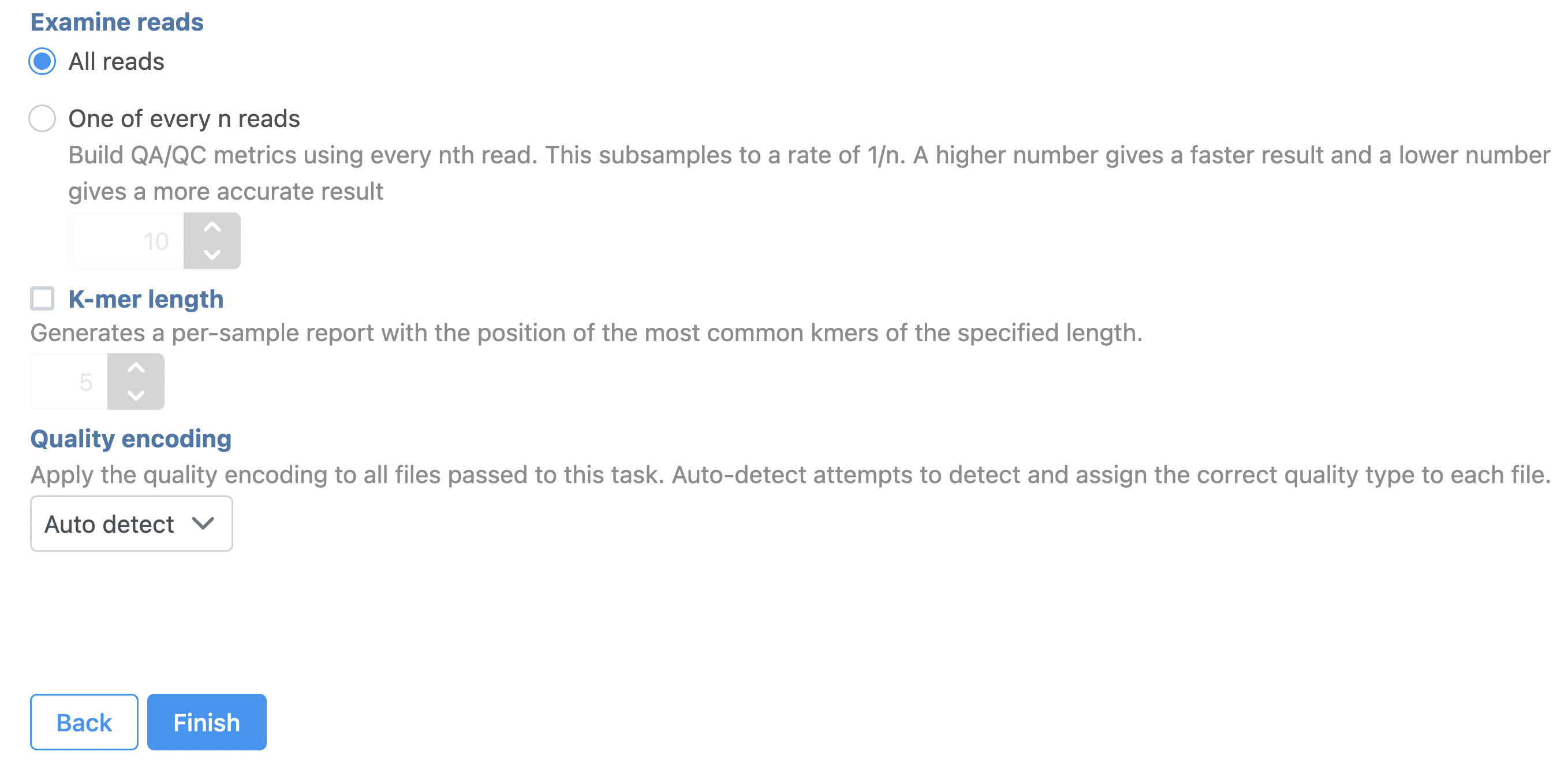
Figure 2. Pre-alignment QA/QC setup dialog (defaults)
Most sequencing applications now use the phred quality score. This score indicates the probability that the base was accurately identified. The table below shows the corresponding base call accuracies for each score:
| Phred Quality Score | Base Call Accuracy |
|---|---|
| 10 | 90% |
| 20 | 99% |
| 30 | 99.9% |
| 40 | 99.99% |
The task report is organised in two tiers. The initial view shows project-level report with all the samples. An overview table is at the top, while matching plots are below.
The Pre-alignment QA/QC output table contains one input file per row, with typical metrics on columns (%GC: fraction of GC content; %N: fraction of no-calls) (Figure 3). The file names are hyperlinks, leading to the sample-level reports. To save the table as a txt file to a local computer, push the Download link. Table columns can be sorted using double arrows icon (![]() ).
).
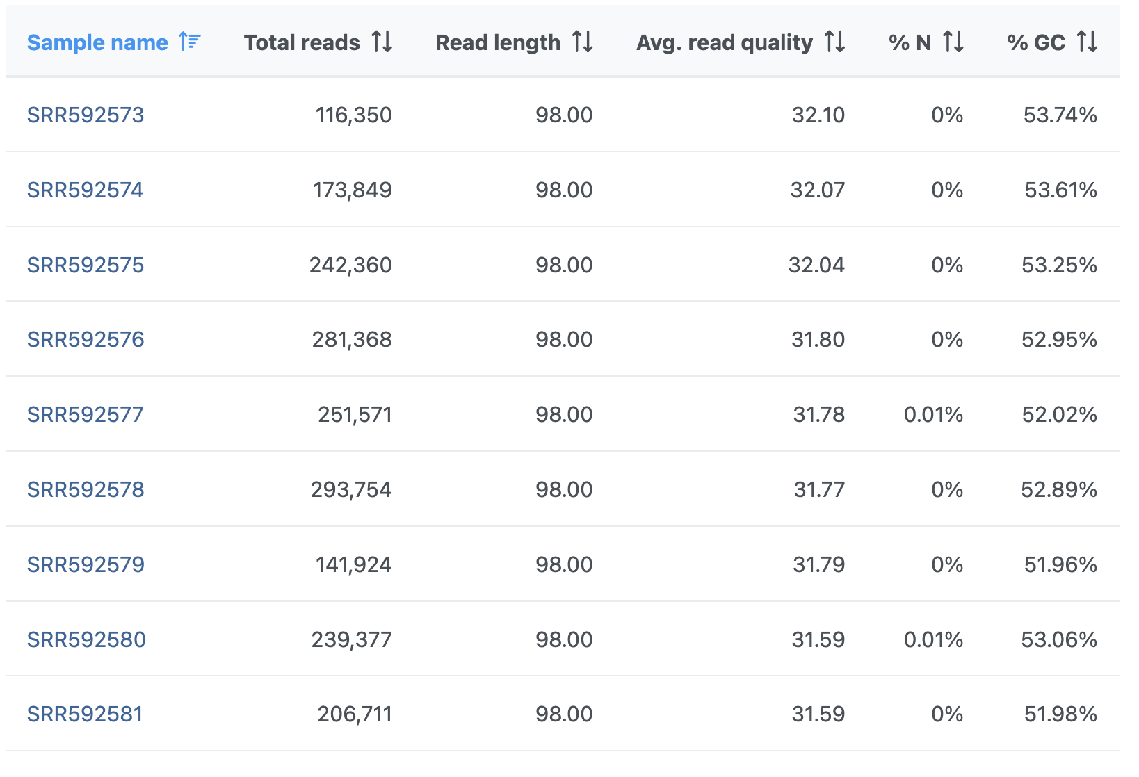
Figure 3. Pre-alignment QA/QC output table (project-level). Each row is an input file. %N: proportion of no-calls, %GC: GC content
Two project-level plots are Average base quality per position and Average base quality score per read (Figure 4). The latter plot presents the proportion of reads (y-axis) with certain average quality score (meaning all the base qualities within a read are averaged; x-axis). Mouse over a data point to get the matching readouts. The Save icon saves the plot in a .svg format to the local machine. Each line on the plot represents a data file and you can select the sample names from the legend to hide/un-hide individual lines.
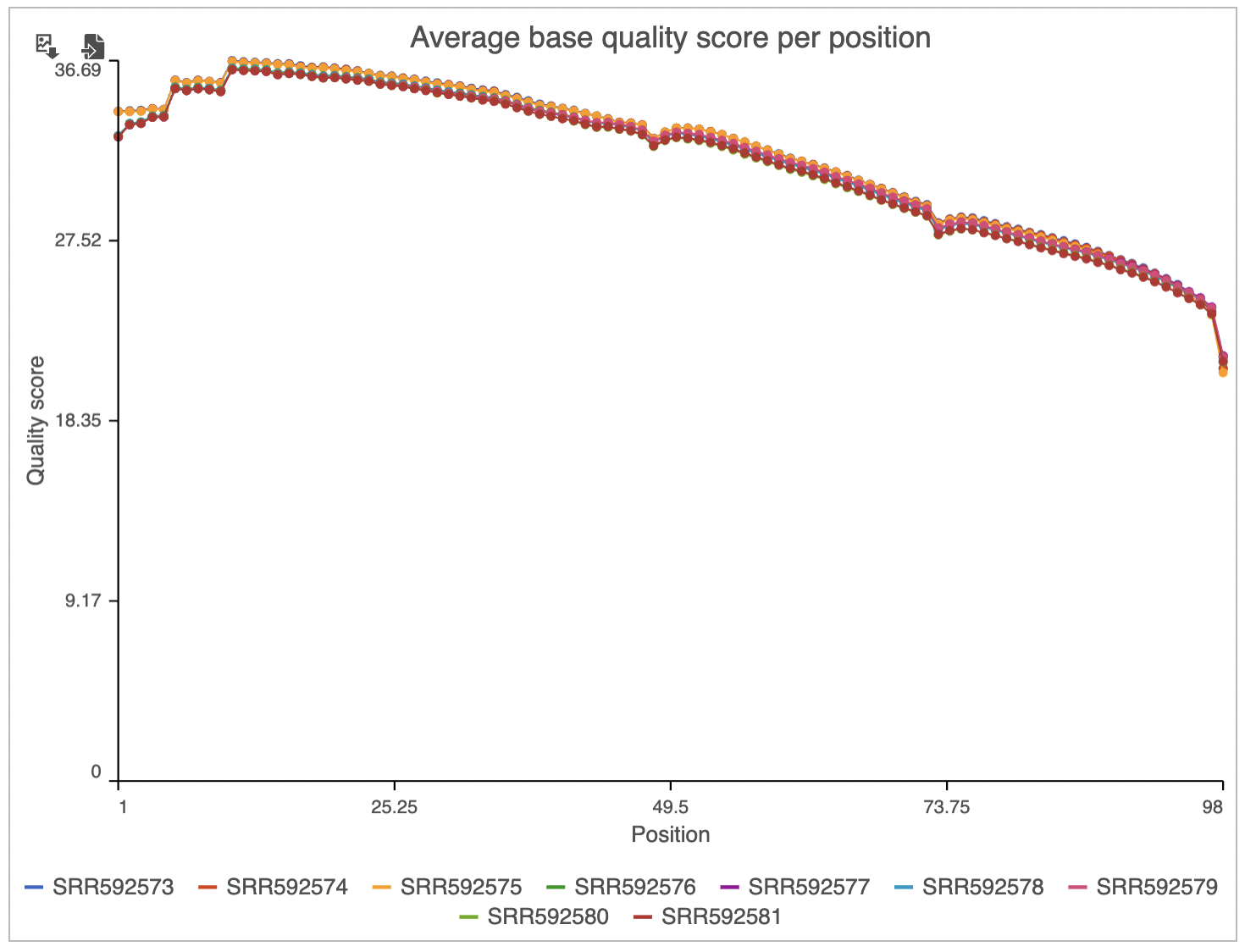
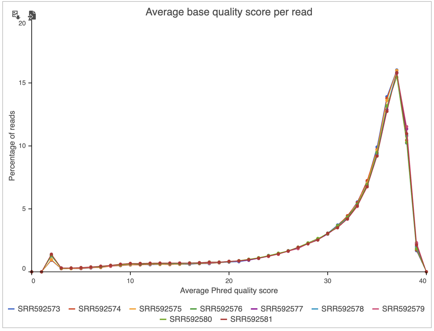
Figure 4. Pre-alignment QA/QC project-level plots (each line is a file)
A sample-level report begins with a header, which is a collection of typical quality metrics (Figure 5).

Figure 5. Header of a sample-level pre-alignment QA/QC report
Below the header you will find four plots: Base composition, Average base quality score per position (same as above, but on the sample level), Distribution of base quality scores (the same as Average base quality score per read, but on the sample level), and Distribution of read lengths.
Base composition plot specifies relative abundance of each base per position (Figure 6), with N standing for no-calls. By selecting individual bases on the legend, you can remove them from the plot / bring them back on. To zoom in, left-click & drag over a region of interest. To zoom out, use the Reset button (![]() ) to recreate the original view, or the magnifier glass (
) to recreate the original view, or the magnifier glass (![]() ) to zoom out one level.
) to zoom out one level.
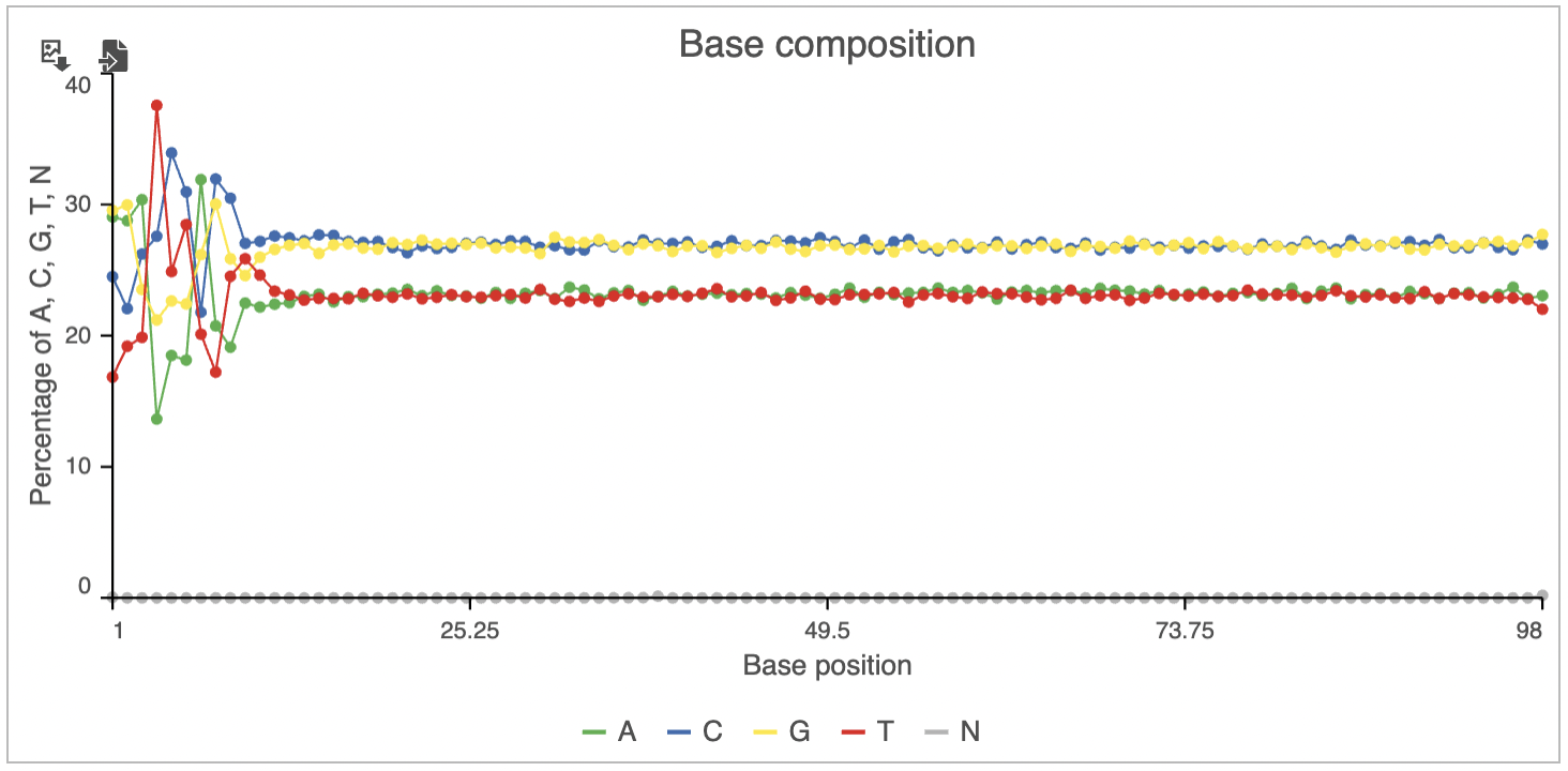
Figure 6. Base composition plot: fraction of each base at a given position within a read. N: no call
Distribution of read lengths shows a single column for fixed length data (e.g. Illumina sequencing). However, for quality-trimmed data or non-fixed length data (like Ion Torrent sequencing), expect to see a read’s length distribution (Figure 7).
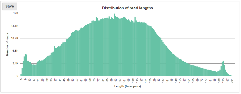
Figure 7. Distribution of read lengths (an example processed by Ion Torrent sequencer is shown)
If K-mer length option was turned on when setting up the task, an additional plot will be added to the sample-level report, i.e. K-mer Content (Figure 8). For each position, K-mer composition is given, but only the top six most frequent K-mers are reported; high frequency of a K-mer at a given site (enrichment) indicates a possible presence of sequencing adapters in the short reads.
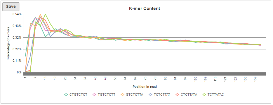
Figure 8. K-mer Content plot. Position of a K-mer is on the horizontal axis, while the K-mer frequency is on the y-axis. Top six K-mers are listed below the plot. In this example, the value of K was set to eight. The most frequent reported K-mer (CTGTCTCT) is a reverse complement of a commonly used adapter (AGAGACAG)
The pre-alignment QA/QC report as described above is generally available for the NGS data of fastq format. For other types of data, the report may differ depending on the availability of information. For example, for fasta format, there is no base quality score information and therefore all the figures or graphs related to base or read quality score will be unavailable.
Additional Assistance
If you need additional assistance, please visit our support page to submit a help ticket or find phone numbers for regional support.


| Your Rating: |
|
Results: |

|
43 | rates |
Overview
Content Tools
1 Comment
Melissa del Rosario
author: ilukic