Hierarchical clustering is a statistical method used to assign similar objects into groups called clusters. It is typically performed on results of statistical analyses, such as a list of significant genes / transcripts, but can also be invoked on the full data set, as a part of exploratory analysis.

Hierarchical clustering is an unsupervised technique, meaning that the number of clusters is not specified up front. In the beginning, each row and/or column is considered a cluster. The two most similar clusters are combined and continue to combine until all objects are in the same cluster. Hierarchical clustering produces a tree (called a dendrogram) that shows the hierarchy of the clusters.

This tutorial will illustrate how to:

Invoking Hierarchical Clustering

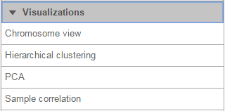
To invoke hierarchical clustering, select a Quantification data node (to cluster samples) or a Feature list data node (to cluster significant genes/transcripts) and then click on the Hierarchical clustering option in the context sensitive menu (Figure 1).

Figure 1. Hierarchical clustering as a part of visualisation tools

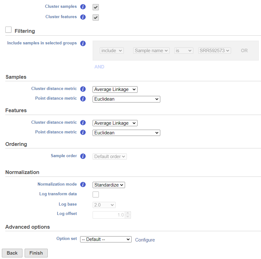
The hierarchical clustering setup dialog (Figure 2) enables you to control the clustering algorithm. Starting from the top, you can choose to Cluster samples, Cluster features (genes/transcripts) or both. By default, if there are less than 3000 samples, the Cluster samples check button is selected, if there are less than 3000 features, the Cluster features check button is selected. Otherwise the check button is de-selected.

Figure 2. Setup dialog of hierarchical clustering (default settings)

Cluster distance metric is used to determine how the distance between two clusters will be calculated. Single Linkage: the distance between two clusters is determined by the distance of the closest objects in the two clusters. Complete Linkage: the distance between two clusters is equal to the distance between the two furthest members of those clusters. Average Linkage: the average distance between all the pairs of objects in the two different clusters is used as the measure of distance between the two clusters. Centroid method: the distance between two clusters is equal to the distance between the centroids of those clusters. Ward's method: the distance between two clusters is designed to minimize the size of an error measure based on the sum of squares.

Point distance metric is used to determine the distance between two rows or columns. For a thorough discussion, we refer you to the distance metrics chapter.

If you do not want to cluster all the samples, but select a subset based on specific sample attributes (i.e. group membership), use the Filtering drop down list (Figure 3). The default value of the Filtering option is All samples.
 

Figure 3. Specifying a subset of data for clustering, based on sample attributes. In the example on the figure, only Control samples will be clustered, while the Treatment samples will be omitted

Customizing the Heat Map

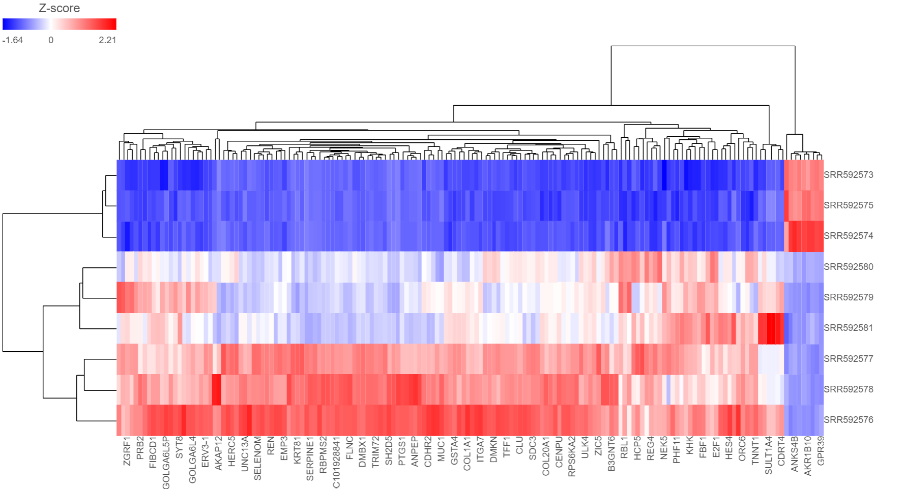
The output of a Hierarchical clustering task is a heat map (Figure 4) with or without dendrogram depends on whether you perform cluster on samples/cells or features. By default, samples are on rows (sample labels are displayed as seen in the Data tab) and features (genes or transcripts, depending on the input data) on columns. Colors are based on standardized expression values (default selection; performed on the fly), with blue indicating low and red indicating high levels of a variable (i.e. low or high expression levels). Dendrograms show clustering of rows (samples) and columns (variables).

Figure 4. Heat map. Samples are on columns, variables (in this example: genes) on columns, and the heat map is based on standardised gene expression values

Depending on the resolution of your screen and number of samples and variables that need to be displayed, some binning may be involved. If there are more than samples/genes than pixels, they will be averaged together. When you zoom in to certain level, you will see each cell represent one sample/gene. To zoom, use the mouse wheel to zoom in / out. To move the map around when zoomed in, press down the right button of the mouse and drag the map.  

To transpose the map, i.e. to see samples on columns and genes on rows, select the Transpose view button( ). To flip rows or columns belonging to the same dendrogram branch, select the flip mode () button.

 When select a cluster by left-clicking & dragging around the dendrogram line in selection mode (), the export button ( will be enabled. Click on it to export the selected features and samples with the normalized values which the heatmap color represents into a text file.

The heat map can be saved as a .svg image by selecting the Save image icon (  ).The control dialog can be seen on Figure 7. The default filename is Dendrogram view.svg and it is downloaded to the local computer.

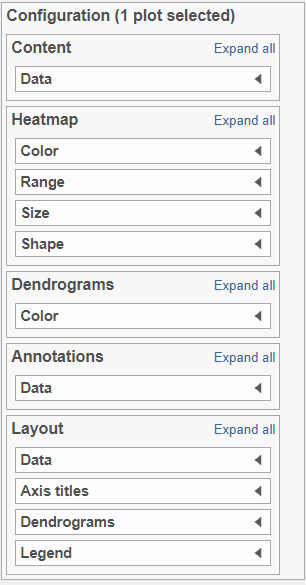
There are 5 sections in the Configuration panel (Figure 5): Content, Heatmap, Dendrograms, Annotations and layout. Click on the triangle () to expand the section to configure.

Figure 5. Heat map controls

Content:

Content contains the value of which matrix data is used to draw heatmap in the plot. Heatmap is a color presentation of the values in the matrix selected. Most of the data nodes contains only one matrix, which you might not need to use Size by configuration to use the same value represent the same information as color by (Figure 6).

Figure 6. When data node contains only one matrix, not need to use size by configuration

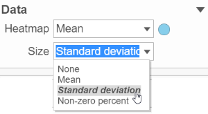
However, if a data node contains multiple matrix information, e.g. if you perform descriptive statistics on cluster groups for every gene like mean, std. dev, percent of detected cells etc, you might want to use color of the component in the heatmap to represent one type of stats (like mean of the groups) and size of component to represent a different statistic information (like std. dev) (Figure 7). 

Figure 7. When a data node containing more than one matrices, use different matrices to color and size the components

Heatmap:

Configure the color of the heatmap is 

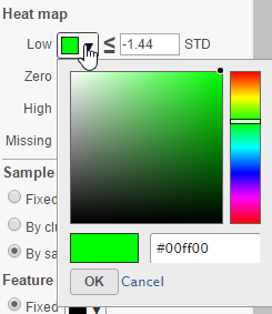
To change a color on the map, click on the arrow head by the color box to get the color mixer (Figure 8). Then pick the color you prefer and select OK. Range of the colors can be changed by typing a different value in the text box to the left of the STD sign (i.e. sandardised).

Figure 8. Color mixer

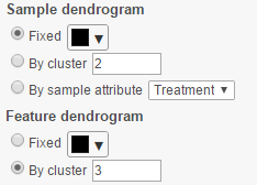
The sample and/or feature dendrogram color can also be configured. By default, the dendrograms are all colored in black (Figure 9 ).

Figure 9. Dendrogram color configuration

When the By cluster radio button is chosen, the number of clusters needs to be specified, and then the top N number of clusters will be in N different colors. For the sample dendrogram, it can also be colored with it's attributes by selecting the By sample attribute radio button and selecting the relevant attribute in the drop-down menu. If the cluster includes samples from different subgroup, the line of the cluster will be mixed color of the subgroup color.

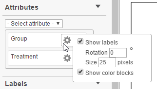
Most of the times you will want to see sample attributes on the heat map. Select the Select attribute drop down list and point to the attribute (as defined in the Data tab) that you want to add to the dendrogram. To remove an attribute from the dendrogram, select the red minus icon (  ). Selecting the gear icon (  ) opens the configuration dialog (Figure 10), which is used to manipulate the dendrogram annotation. Group labels can be turned on or off (Show labels), rotated (Rotation) or re-sized (Size). The color blocks around the labels can also be turned on or off (Show color blocks).

Figure 10. Configuring group attributes on the dendrogram

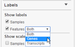
The Labels section of the control panel deals with different labels. First, Show labels turns sample and feature labels on or off. For features with both gene- and transcript level-information, click on the drop-down menu to select which you would like to display, by default, both are shown (Figure 11). 

Figure 11. Select in the drop-down menu whether to display gene- or transcript level information

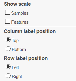
If needed, scales for sample or feature dendrograms can also be added (Show scale). Column labels can be placed at the Top or at the Bottom, while Row labels can be on the Left or on the Right (Figure 12).

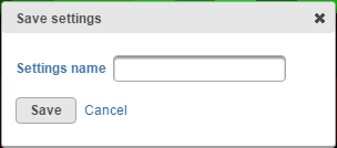
Commonly used plot customization can be saved by selecting the Save settings button. Give your setting set a name (Figure 13) and select Save. Saved settings will be available under the Saved settings list, and can be deleted by clicking on the red cross button(  ). To revert to manufacturer settings at any time, use the Default settings hyperlink.

Figure 13. Saving heat map settings

Your Rating:

Thanks for voting!

Please Wait

Results:

4

rates