Lists

Scientists often develop lists of genes, probes, transcripts, SNPs, and genomic regions of interest from analysis tools, research papers, and databases. Using Partek^® Genomics Suite^®, these lists can be integrated with genomics data sets, analyzed with powerful statistics, and visualized for new insights.

This tutorial will illustrate:

Importing a text file list

The preferred method for importing a generic list of data into Partek Genomics Suite is as a text file.

Select File from the main toolbar
Select Text (.csv .txt)...under the Import option
Select the text file to launch the Import .txt, .tsv, or .csv File dialog

The File Type section of the Import dialog includes a preview of the text file and import options (Figure 1).

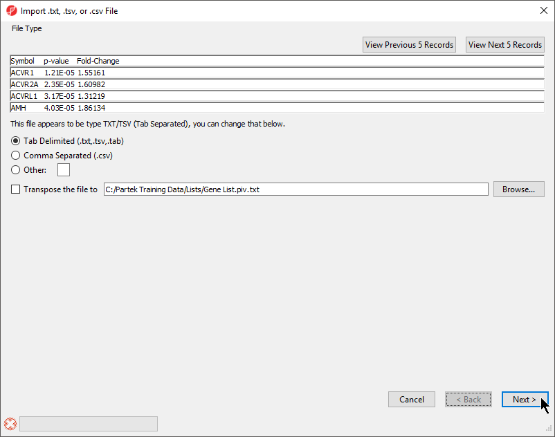
Figure 1. Import .txt, .tsv, or .csv file dialog

The columns in the import file can be separate by a tab, comma, or any other character.

For most applications, the items on the list should be in rows while attributes or values should be in columns. If a list is oriented with items on columns, select Transpose the file to to import a transposed spreadsheet.

Select Next > to move to the Data Type section
Select your data type; here we have chosen Genomic Data because it is a gene list (Figure 2)

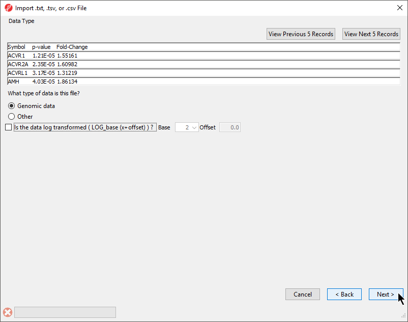
Figure 2. Selecting the data type

Selecting Genomic Data will result in a dialog prompt to configure genomic properties including selecting the type of genomic data, the location of genomic features in the spreadsheet, the annotation column with gene symbols, the chip or reference source and annotation file, and the species and genome build. This option should be selected if the text file contains genomic position data or other array/sequencing results.

Select Next >

The Identify Column Labels, Start of Data section (Figure 3)

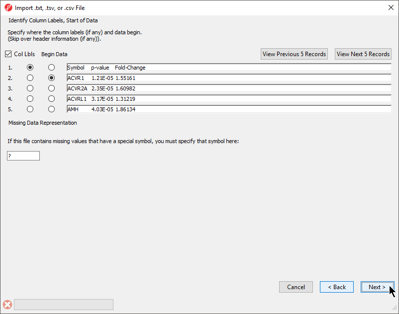
Figure 3. Identifying column labels and start of data

The next step is to identify where the data starts and where the optional header is found. The line that contains the header (if present) must precede the data. If there are lines to be skipped in the file (like comments), they may only appear at the top of the file, before the header line or data begin.

If there are many comment lines at the start of the file, you may need to select View Next 5 Records to get to the row that contains the column header. If you accidentally move past the screen that contains the header or data rows, select View Previous 5 Records.

If there are missing numerical values or empty cells in your input list, insert a special character or symbol (?, N/A, NA, etc.) in the missing cells; you will specify the character in the Missing Data Representation section of the dialog

If a header row is present, select Col Lbls to allow you to select a column header row
Select the row where the data beings using the Begin Data selector
If any cells have a missing value, you can signify this with a special symbol selected using the Missing Data Representation panel

This is important if the missing value is a number in a column that you plan to use for statistical analysis. The default missing value indicator is ?.

Select Next >

The Preview text encoding section (Figure 4) previews the first five lines of the file, allowing you to check if the text encoding is correct.

If the text does not appear properly, use the Specify the text encoding: drop-down menu to choose the correct encoding

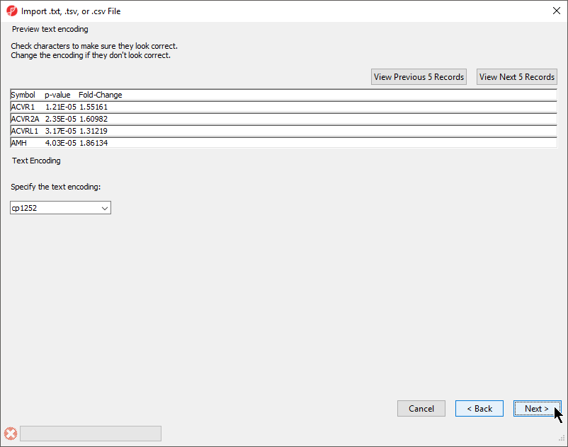
Figure 4. Previewing text encoding

Select Next >

The final section of the Import .txt, .tsv, or .csv File dialog is Verify Type & Attribute of Data Columns (Figure 5). While data column type and attribute can be modified after import, it is easier and faster to select the proper options during import as multiple columns may be selected during this dialog.

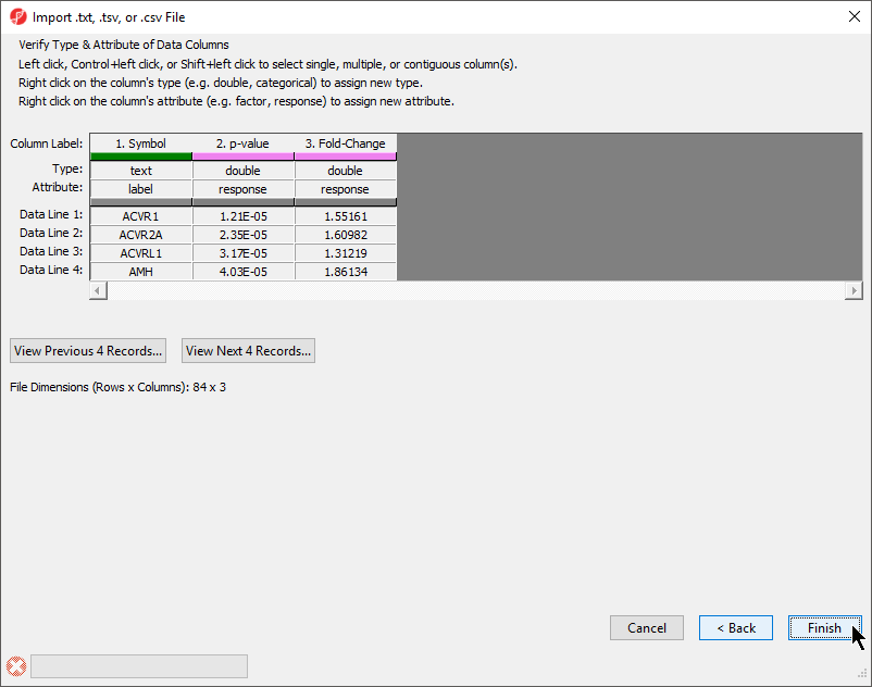
Figure 5. Verifying type and attribute of data columns. While individual column types and attributes can be modified after import, this dialog allows multiple columns to be selected and modified simultaneously.

Check and modify column types and attributes

If there is an identifier like gene symbol or SNP, the Type field for that column should be set to text and Attribute should be set to label. Numeric values (intensities, p-values, fold-changes, etc.) should have Type set to double and Attribute set to response. The other possible value for Attribute is factor and describes sample data. The user interface is this dialog allows you to select multiple columns at once. The interface controls are detailed in the dialog (Figure 5).

Select Finish to import the text file and open it as a spreadsheet

If Genomic Data was selected in the Data Type section, the Configure Genomic Properties dialog will open (Figure 6). These options will be discussed in the next section when we add an annotation file, but we will make a few selections now.

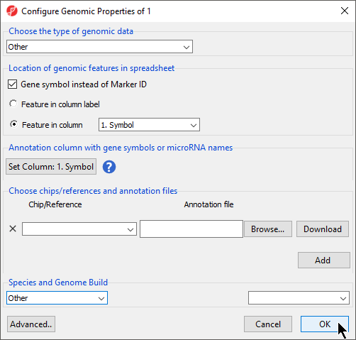Figure 6. Many types of genomic data can be imported into Partek Genomics Suite using the text data file importer. This dialog allows these files to be associated with an annotation file and reference genome.

Select Other from the Choose the type of genomic data drop-down menu
Select Gene symbol instead of Marker ID
Select Feature in column and choose Symbol from the drop-down menu
Set Column 1. Symbol will be automatically selected
Select OK

The imported spreadsheet will open (Figure 7).

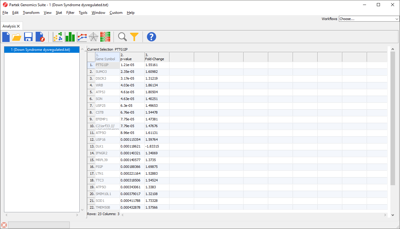
Figure 7. An imported .txt data file spreadsheet

Tasks available for a list of genes

There are many useful visualizations, annotations, and biological interpretations that can operate on a gene list. In order for these features operate on an imported list, an annotation file must first be associated with the gene-list. Additionally, many operations that work with a list of significant genes (like GO- or Pathway-Enrichment) require comparison against a background of “non-significant” genes.

Adding an annotation file

The quickest way to accomplish both is to use the background of “all genes” for that organism provided by an annotation source like RefSeq, Ensembl, etc. in .pannot (Partek^® annotation), .gff, .gtf, .bed, tab- or comma-delimited format. If the file is not already in a tab-separated or comma delimited format, you may import, modify, and save the file in the proper file format.

Select File from the main toolbar
Select Genomic Database under Import
Select the annotation file; we have selected hg19_refseq_14_01_03_v2.pannot from the C:/Microarry Libraries folder
Delete or rearrange the columns as necessary; we have placed the column with identifiers that correspond to our gene list first
Select () to save the annotation file; we have named it Annotation File
Select () to close the annotation file

Now we can add the annotation file to our imported gene list.

Right click 1 (Gene List.txt) in the spreadsheet tree
Select Properties from the pop-up menu

This is the Configure Genomic Properties dialog we saw earlier (Figure 6).

Select Browse under Annotation File
Choose the annotation file; we have chosen Annotation File.txt
Select appropriate species and genome build options; we have selected Homo sapiens and hg19
Select OK

Adding annotations

Inserting annotations from an annotation file

If a genomic annotation file has been added, annotations from the file can be added as columns in the spreadsheet.

Right click on a column header
Select Insert Annotation
Select columns to add from Column Configuration (Figure 8)
Select OK

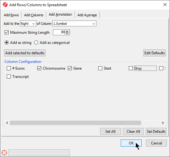
Figure 8. Adding an annotation column from the annotation file

Annotating with cytobands

Select Annotate with Cytobands from Tools in the main toolbar when a suitable spreadsheet is open

A column with cytoband locations will be added to the spreadsheet. Adding a cytoband is possible if genomic coordinates are associated with the gene list spreadsheet during import or by association with an annotation file.

Annotating with known SNPs

Select Annotate with Known SNPs from Tools in the main toolbar when a suitable spreadsheet is open will add

A column of SNPs associated the listed genes and a column indicating the number of SNPs known to be associated with the genes will be added to the spreadsheet. If a SNP database has not been previously downloaded, it will need to be downloaded through the SNP database dialog (Figure 9).

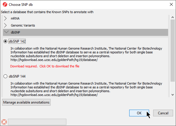
Figure 9. Choosing a database source for annotating a list of genes or genomic coordinates

Alternatively, to generate a list of SNP IDs per row, right-click on a row header and select Create list of dbSNP.

In addition to SNPs, this feature can associate any data with a list of genes or genomic coordinates; the dbSNP database, any miRNA database, data from the Database of Genomic Variants (dgv), any mRNA transcriptome database, or any custom annotation source can be associated with your list. In each case, this feature will add columns to the imported gene list spreadsheet that match the genes with features from those databases.

GO Enrichment

The Gene Ontology (GO) Enrichment p-value calculation uses either a Chi-Square or Fisher’s Exact test to compare the genes included in the significant gene list to all possible genes present in the experiment or the background genes. For a microarray experiment, background genes consists of all genes on the chip/array; for a next generation sequencing experiment, all genes in the species transcriptome are considered background genes.

Because the calculation is essentially comparing overlapping sets of genes and does not use intensity values, GO Enrichment can be performed on an imported gene list. GO Enrichment is available through the Gene Expression workflow.

If no annotation file has been specified for the gene list, GO Enrichment will use the full species transcriptome as the background genes. While suitable for next generation sequencing experiments, for microarray experiments, only the genes on the chip/array are appropriate. Please contact our technical support department for assistance with this step if needed.

Pathway Enrichment

Like GO Enrichment, Pathway Enrichment does not require numerical values, but instead operates on lists of genes - a list of significant genes vs. background genes. Consequently, Pathway Enrichment may be used with an imported list of genes. The list of background genes is set to the species transcriptome by default, but can be set to a specific set of genes if the gene list has been associated with an annotation file.

Tasks available for a gene list with numeric data

All the operations available for a gene list are available; you may also use the numeric data associated with the genes for visualization, clustering, and statistical operations.

Descriptive Statistics

There are numerous descriptive statistics available in Partek Genomics Suite.

Select Stat from the main toolbar
Select either Descriptive or Correlate to show available options

Principal Component Analysis is located in a different menu.

Select Tools from the main toolbar
Select Discover
Select Principal Component Analysis

Applying Multiple Test Correction

If your imported data contains a list of p-values, you can use any of the available multiple test corrections.

Select Stat from the main toolbar
Select Multiple Test
Select Multiple Test Corrections to launch a dialog with available options

Plotting numeric data associated with a gene list

A variety of profile plots can be used to visualize the numerical data associated with your imported gene list.

Select View from the main toolbar
Select any applicable option

Genome Browser

If you have imported numerical data associated with genes (like p-values or fold-changes), you can visualize these values in the Genome Browser once an annotation file has been added.

Right-click on a row header in the imported gene list spreadsheet
Select Browse to location

If the annotations have been configured properly, you should see a track for the first column of numerical data, a cytoband track, and an annotation track. You can also add another track to display a second column of numerical data.

Select New Track
Select Add a track from spreadsheet
Select Next >

A new track titled Regions will be added.

Select Regions in the track preferences panel to edit it
Select the other numerical column in the Bar height by drop-down menu

Clustering

If the data is suitable for clustering, access the clustering function through the toolbar, not form a workflow. The workflow implementation assumes the data to be clustered are found on a parent spreadsheet and the list of genes is in a child spreadsheet. Because the data to be clustered is all on one spreadsheet, access hierarchical clustering by selecting Tools from the main toolbar then Discover then Hierarchical Clustering. Consider transposing the spreadsheet if samples are on columns and genes are on rows as Hierarchical Clustering will assume samples are rows and genes are columns. If you only have one column or one row of data, cluster only on the dimension with multiple entries by deselecting either Rows or Columns from What to Cluster or consider using an intensity plot instead.

Starting with a list of SNPs

A list of SNPs using dbSNP IDs can be imported as a text file and associated with an annotation file as described for a list of genes. The annotation file (genomic database) you use to annotate the SNPs should minimally contain the genomic coordinates (chromosome number and physical position) of the locus.

Novel SNPs, or SNPs that are not found in your annotation source, must be imported as a region list. The only difference would be to use the SNP name in place of a region name.

Annotating SNPs with genes

Starting with a list of SNPs that have been associated with genomic loci using an annotation file and assigned a species with genome build, you may use Find Overlapping Genes to annotate these SNPs with the closest genes.

Select Tools from the main toolbar
Select Find Overlapping Genes
Select Add a New Column with the Gene Nearest to the Region from the method dialog

The Report Regions from the specified database dialog will open.

Select your preferred database
Select OK

This will add 3 columns to the list of SNPs spreadsheet including Nearest Feature, which will indicate the nearest gene and strand. To allow gene list operations such as GO Enrichment or Pathway Enrichment to be performed on the SNP list, we can set the Nearest Feature column as the Gene Symbol column.

Right click the spreadsheet in the spreadsheet tree
Select Properties from the pop-up menu
Select Gene symbol instead of Marker ID
Select Feature in column and select Nearest Feature
Select OK

Annotating a Partek Genomics Suite-generated SNP list with SNVs

If you have a SNP spreadsheet that was generated using Partek Genomics Suite, you can annotate the SNP list with gene, transcript, exon, and information about the predicted effect of the SNPs.

Select Tools from the main command toolbar
Select Annotate SNVs

Starting with a list of genomic regions

Importing a region list

A region list in PGS must contain the chromosome, start location, and stop locations as the first three columns, respectively. The chromosome name (or number) in the region list must be compatible with the genomic annotation for the species if you plan to use any feature (like motif detection) that requires reference sequence information.

Import the region list as described above for text files. Select Other for data type. Chromosome name or number should be imported as a text field; location start and stop may be either integer or text.
Right-click on the imported spreadsheet in the spreadsheet tree
Select Properties
Select List of genomic regions from the Configure Spreadsheet dialog
Select region in the Add Property drop-down menu and select Add

The spreadsheet properties will now include region. If you would like to do any operation that requires looking up hte reference genomic sequence information for the regions based on genomic location, you will need to specify the species for this region list.

Right-click on the imported spreadsheet in the spreadsheet tree
Select Properties
Select Genomic from the Add Property drop-down menu
Select Add
Select your options from the Species and Genome Guild drop down menus
Select OK

With a few additional options, the region list can be made viewable in the genome browser.

Right-click on the imported spreadsheet in the spreadsheet tree
Select Properties
Select Advanced..
Select Edit next to the species name
Specify the Cytoband file and 2Bit sequence file
Select OK

Motif detection

Starting with a region list, you may detect either known or de novo motifs using the ChIP-Seq
workflow if your spreadsheet has been associated with a species and a reference genome as
described in the import section.

Select ChIP-Seq from the Workflows drop-down menu
Select Motif detection from the Peak Analysis section of the workflow

Both options (Discover de novo motifs and Search for known motifs) can now be performed. Motifs (de novo) may be displayed in the Genome Browser and known detected motifs may be viewed in web-log format by right-clicking on a header row of the motif spreadsheet.

Determining the average values for a region list

If you have a region list or a bed file and you have a microarray experiment with data, you can summarize the data according to the genomic coordinates contained in the region list. For instance, the region list contains a list of CpG islands, the experiment contains methylation percentage values for probes (β values), and you would like to summarize the methylation values for individual probes for the CpG islands. Or you have a list of copy number amplifications, microarray gene expression data, and you are interested in determining if the average intensities of the probes in those regions is higher than expected.

Import the region list (or BED file) and specify the region property as explained elsewhere in this document
With the region list spreadsheet selected, right-click in any column header and select Insert Average
A dialog box similar to that shown. With the Add Average tab selected, specify the location where you like the new columns to appear by using the Add to the and of Column pull-down menus. Specify the top-level spreadsheet containing the data you wish to be averaged (β values, gene-intensity values, etc.) in the Get average from spreadsheet pull-down menu. Choose the radio button to specify how the averaging should be done. The bottom two choices (Mean of all samples and Mean value for all samples separately) are obvious; the first option (Mean of samples significant in region) is used when the region list has a SampleID associated with each region. In this case, the column designated as the SampleID column from the top-level spreadsheet will be used to identify the sample to be summarized for each region.

Find region overlaps

You have a list of regions from another analysis program (perhaps you detected peaks using an R program) and you’d like to compare that region list with a region list that Genomics Suite calculated. Perhaps you have two lists created by Genomics Suite (one generated from peak detection with one set of parameters and the other created with different parameters) and you’d like to see what the two lists have in common. You may use the Tools > Find Region Overlaps command to compare two or more region lists as shown.

There are two separate modes of operation for this command: Report all regions and Only report regions present in all list. The first option, Report all regions, will report all regions in both lists. If there is any region overlap between the lists, the intersection of the regions will be reported along with the start and stop coordinates of the intersection, the percent overlap between the intersected region with each of the regions in the input lists. If a region is found in only one list, it will be reported as well.

In contrast, the second option, Only report regions present in all lists, will intersect both lists and only reports regions found in all the lists.

Importing genomic locations to be used with annotating SNVs

The Tools > Annotate SNVs feature requires four columns of data per genomic location: the position of the SNP (chr.basePosition), the SampleName, a reference base, and the SNP call (single nucleotide or genotype) as shown in Figure 20.

Prepare input list as shown in Figure 20 and save as either a tab-separated or comma separated
file
Use File > Import > Text to import the table. During import, change the data type of column 1 (as in Figure 3) to text by right-clicking on the color bar of column one and changing the data type to text. You may leave the other columns as categorical response types
The correct properties must be set for this spreadsheet. Right-click on the newly imported spreadsheet in the navigator and select Properties
Choose Other in the Configure Spreadsheet dialog (Figure 6)
Make sure Genomic is selected in the Add Property pull-down menu and select Add In the next dialog box, select Genomic location instead of marker IDs in the Choose the type of genomic data. The Marker ID in column should be set to the first column. [If Marker ID in column does not contain any items in the pull-down list, it is likely that the first column was not a text column (drawn in gray) during import. If this happens, then right-click in the column header in the spreadsheet and change Type: to text.]
Specify the Species from a pull-down menu selection or by typing in the species name. Select Edit Genome to specify the Species Name, Genome Version, Cytoband file, and 2Bit sequence file. The last two fields are optional. Select OK

Now that the properties have been set appropriately, Tools > Annotate SNVs may be invoked on this
spreadsheet.

Importing a BED file

A BED (Browser Extensible Data) file is a special case of a region list: it is a tab-delimited text file and the first three columns of BED files contain the chromosome, start, and stop locations. To import a bed file to be used as a data region list, follow the import instructions for region lists. A BED File might also be visualized as an annotation file containing regions in the Genome Browser.

Using a BED file as an annotation source for the genome browser

BED files do not contain individual sequences nor do the regions have names. For instance, the UCSC table browser has a BED file that contains reads from a long non-coding RNA-Seq experiment and you might like to view this information in the context of your dataset. Before you could visualize a BED file in the chromosome viewer, you would have to create a Partek annotation file from the BED file.

From the top command menu, select Tools > Annotation Manager
In the My Annotations tab, select Create Annotation
Select BED file (.bed) under Choose Annotation Type
Under File Locations, specify the Source (input BED file) with the Browse menu item. You may also specify the Result file name (of the annotation file) and location with the Browse button. You might consider saving the result file to your Microarray Libraries folder
In the Annotation Details section of the dialog box, specify the Name of the annotation database that will be visible from within Genomics Suite, Species, and Genome Build. Preview Chromosome Names would be used if the chromosome names in the annotation file must be changed to match the name of the chromosome in the genomic annotations.
Select OK

Visualizing a BED file as an annotation track in the genome browser

In order to use a BED file as an Annotation track in the Genome Browser, first create the annotation file as described above, being careful to have specified the species and genome build appropriately.

Invoke the Genome Browser by right-clicking in any spreadsheet that has genomic features on rows (gene lists, ANOVA results, SNP detection) and select either Browse to Row or Browse to Location
In the Track Toolbar on the left, select New Track which invokes the dialog shown in Figure 21
Select Add an annotation track with genomic features from a selected annotation source and select Next
Next you will have to choose the annotation file that was created from the BED file. The procedure for doing this might vary slightly depending on the type of spreadsheet you have displayed in the Genome Browser. You may be shown a list of annotations that includes the annotation source you have created; in this case, select the radio button in the Available Annotations panel. If, however,
At the bottom of the screen, you should either check or uncheck the box next to Separate strands (checking means that the BED file contained the strand information for each region and you wish to visualize the regions on different strands). Unselecting Separate strands should be used if the BED file did not contain strand information or if you do not wish to display the information on separate strands. Select Create

GO ANOVA, GSEA/GeneSet ANOVA, and Pathway ANOVA

As these features require intensity (or count) data as well as experimental groups, these features cannot be performed on an imported lists.

Integrating Imported Data

If the data from imported spreadsheets has been associated with annotations, several integration approaches may be used to integrate multiple kinds of imported data. For instance, the Genome Browser may be used to display data from multiple spreadsheets/experiments regardless of the type of spreadsheets (imported data or microarray or NGS experiments). The Venn Diagram tool may be used to find overlaps based on a feature name. Tools > Find Overlapping Regions can use an imported gene list and a list of regions from a copy number or ChIP-Seq experiment to identifygenomic regions in common.

Additional Assistance

If you need additional assistance, please visit our support page to submit a help ticket or find phone numbers for regional support.

Your Rating:

Results:

0

rates

PGS Documentation

Page tree