Page History
...
| Numbered figure captions | ||||
|---|---|---|---|---|
| ||||
|
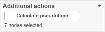
As a result, the cells will be annotated by pseudotime, using green to red gradient (start and end, respectively) (Figure xxx). If, for a particular tree, no root node has been specified, those cells will be omitted from the pseudotime calculation and will be colored in gray (not shown).
| Numbered figure captions | ||||
|---|---|---|---|---|
| ||||
|

As a result of pseudotime calculation, three types of cell nodes will become apparent on the plot.
Root node (white). Root nodes are start points of the pseudotime and were defined by the user in the previous step (e.g. node 7 in Figure xxx).
Branch node (black). Branch nodes indicate where the trajectory tree forks out; i.e. each branch represents a different cell fate or different trajectory (e.g. nodes 1 and 4 in Figure xxx).
Leaf (light gray). Leaves correspond to different cell fates / different trajectory outcomes (e.g. nodes 3, 8, and 11 in Figure xxx). The leaves correspond to cell states of Monocle 2.
| Numbered figure captions | ||||
|---|---|---|---|---|
| ||||
|

| Additional assistance |
|---|
| Rate Macro | ||
|---|---|---|
|
...
Overview
Content Tools