Join us for a webinar: The complexities of spatial multiomics unraveled
May 2
Page History
...
| Numbered figure captions | ||||
|---|---|---|---|---|
| ||||
|
388pxA PCA task node will be added to the pipeline under the Analyses tab and a circular PCA output data node will be produced (Figure 2).
...
| Numbered figure captions | ||||
|---|---|---|---|---|
| ||||
|
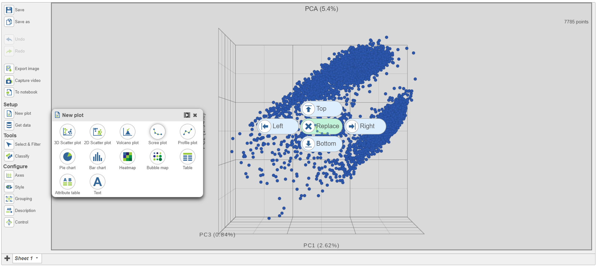
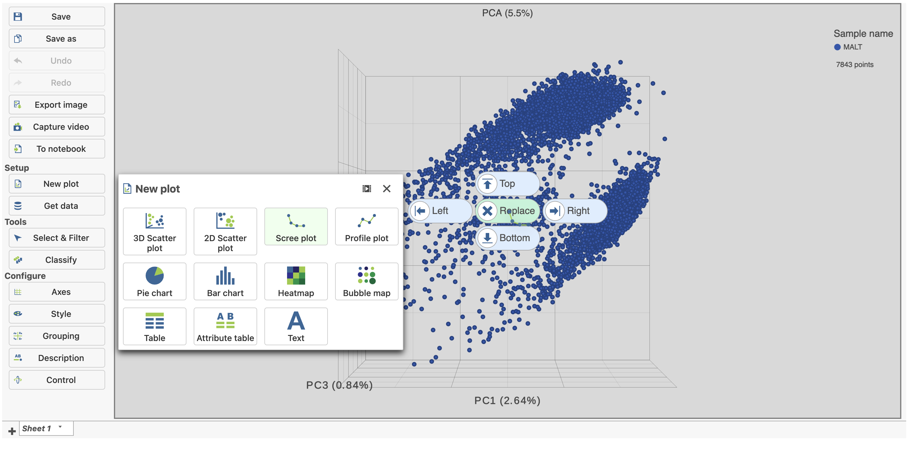
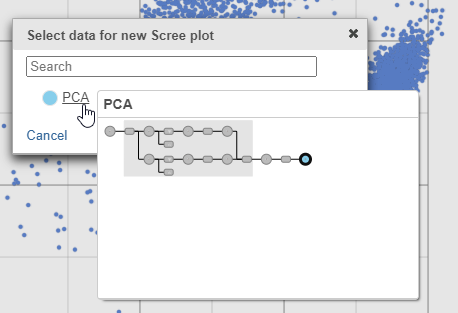
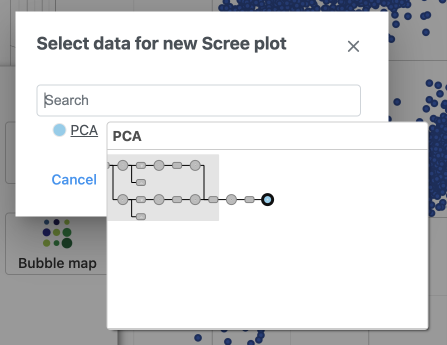
- Select PCA as data for the new Scree plot (Figure 5)
...
| Numbered figure captions | ||||
|---|---|---|---|---|
| ||||
|
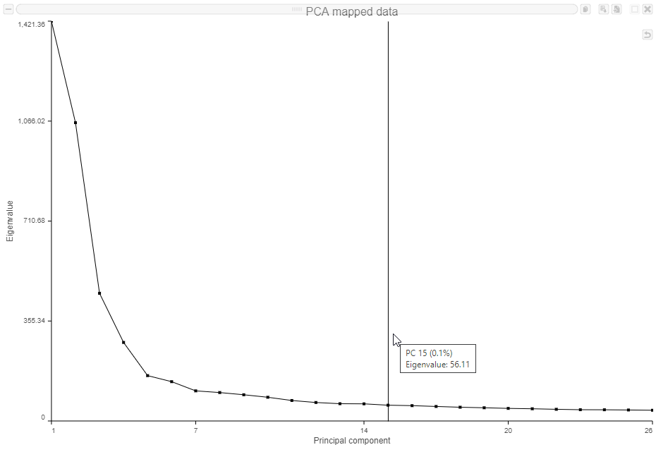
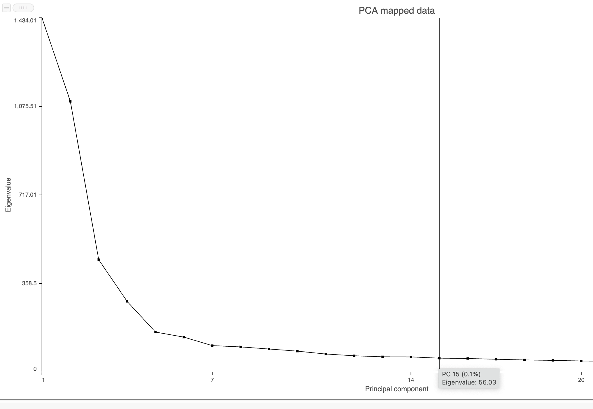
The Scree plot (Figure 6) shows the eigenvalues on the y-axis for each of the 100 PCs on the x-axis. The higher the eigenvalue, the more variance explained by each PC. Typically, after an initial set of highly informative PCs, the amount of variance explained by analyzing additional components is minimal. By identifying the point where the Scree plot levels off, you can choose an optimal number of PCs to use in downstream analysis steps like graph-based clustering and UMAP.
...
| Numbered figure captions | ||||
|---|---|---|---|---|
| ||||
|
Graph-based clustering
...
| Numbered figure captions | ||||
|---|---|---|---|---|
| ||||
|
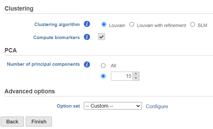
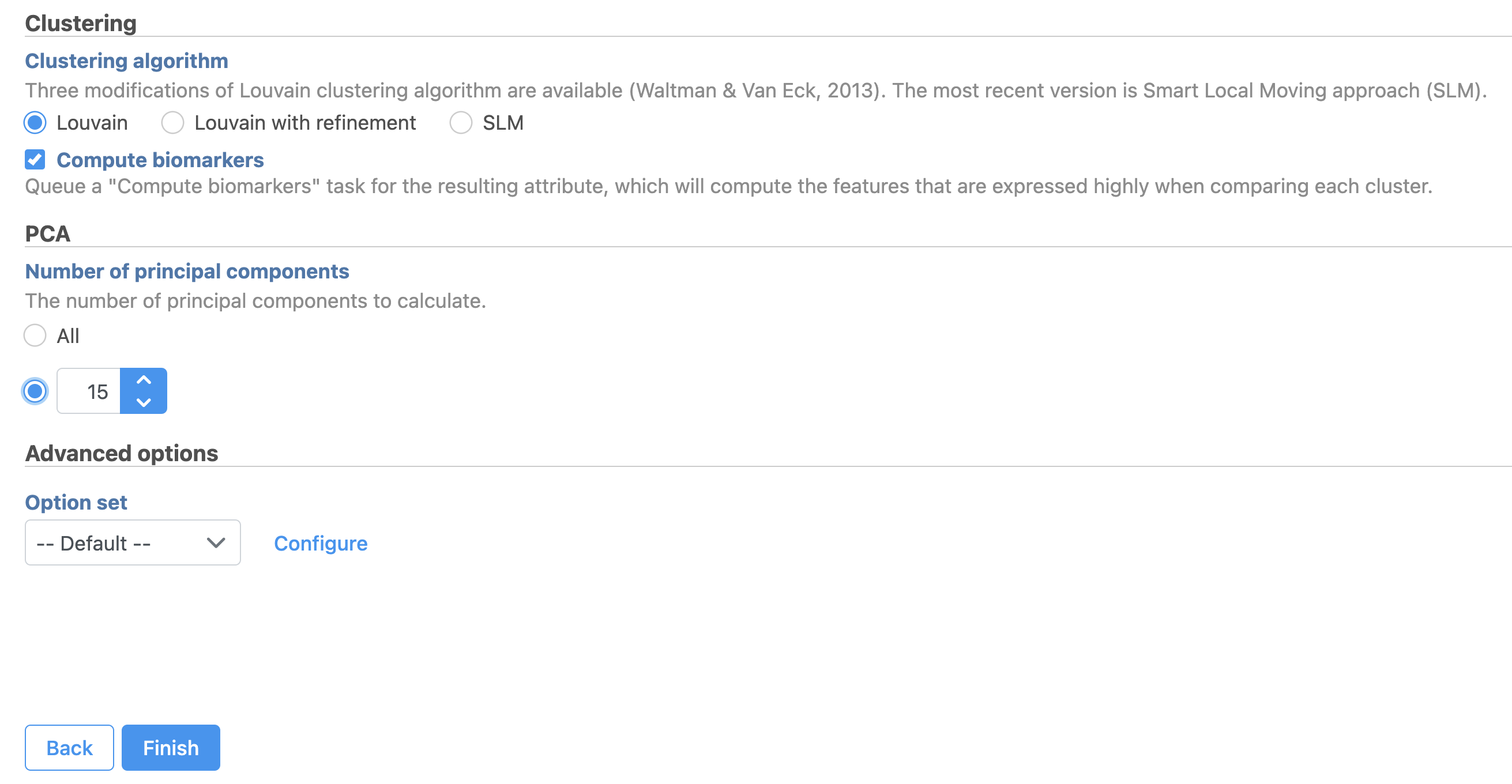
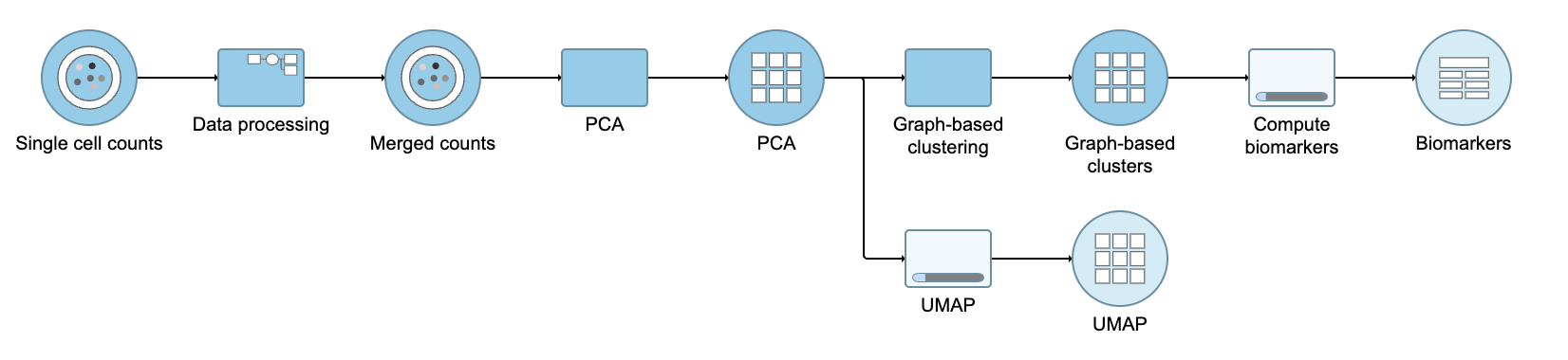
A Graph-based clustering task node will be added to the pipeline under the Analyses tab and a circular Graph-based clusters output data node will be produced (Figure 10)
...
| Numbered figure captions | ||||
|---|---|---|---|---|
| ||||
|

UMAP
Once the graph-based clustering task has completed, we can visualize the results with a UMAP plot. You could use the same steps here to generate a t-SNE plot. For this tutorial, we will use UMAP, as it is faster on several thousand cells.
- Click the circular Graph-based clusterscircular PCA data node
- Click Exploratory analysis in the toolbox
- Click UMAP
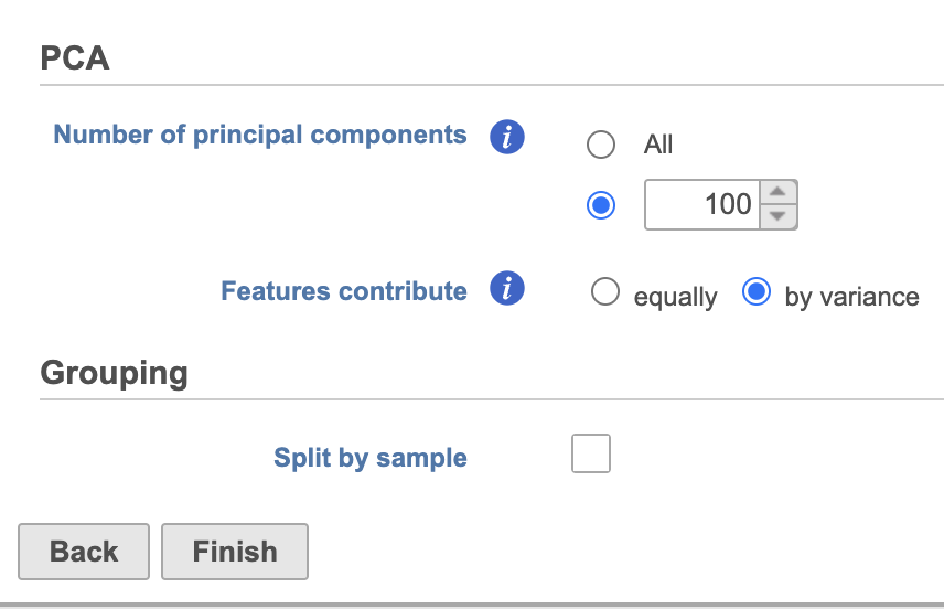
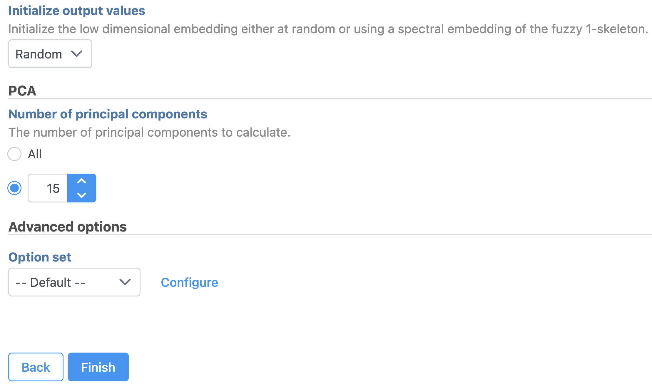
- Set the number of principal components to 15 (Figure 11)
- Click Finish to run the task
...
| Numbered figure captions | ||||
|---|---|---|---|---|
| ||||
|
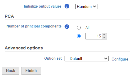
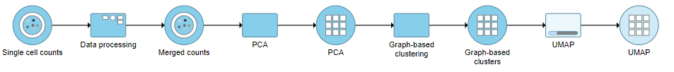
A UMAP task node will be added to the pipeline under the Analyses tab and a circular UMAP output data node will be produced (Figure 12)
...
| Numbered figure captions | ||||
|---|---|---|---|---|
| ||||
|
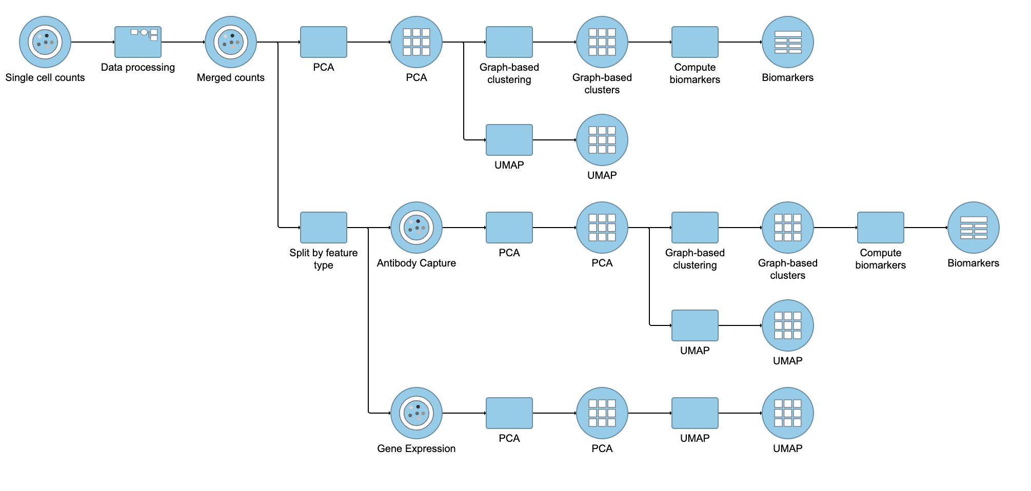
Notes on Performing Exploratory Analysis with Protein or Gene Expression Data Only
...
| Numbered figure captions | ||||
|---|---|---|---|---|
| ||||
|
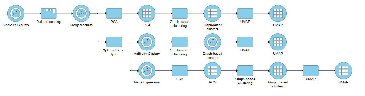
You can then use the Data viewer to bring together multiple plots for comparison (Figure 14).
...
Overview
Content Tools