Page History
...
- Store the 16 .idat files
...
- at C:\Partek Training Data\Differential Methylation Analysis or to a directory of your choosing. We recommend creating a dedicated folder for the tutorial.
- Go to the Workflows drop down list, select Methylation (Figure 1)
| Numbered figure captions | ||||
|---|---|---|---|---|
| ||||
|

- Select Illumina BeadArray Methylation from the Methylation sub-workflows panel (Figure 2)
| Numbered figure captions | ||||
|---|---|---|---|---|
| ||||
|

- That will open Illumina BeadArray Methylation workflow (Figure 3)
| Numbered figure captions | ||||
|---|---|---|---|---|
| ||||
|

- Select Import Illumina Methylation Data to bring up the Load Methylation Data dialog
- Select Import human methylation 450/850 .idat files (Figure 54)
| Numbered figure captions | ||||
|---|---|---|---|---|
| ||||
|
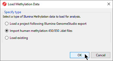
- Select OK
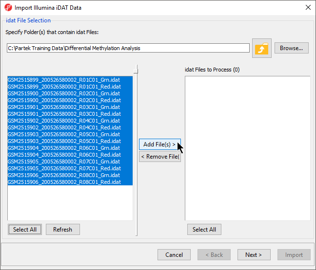
- Select Browse... to navigate to the folder where you saved stored the .idat files
All .idat files
...
in the folder will be selected by default (Figure 5).
| Numbered figure captions | |
|---|---|
|
...
|
...
|
...

...
In the next dialog, use Browse… to point to the folder in which the .idat files were unzipped and use the Add File > button to move the .idat files to the box on the right (i.e. idat Files to Process; Figure 2). Select Next > to proceed.
...
|
- Select Add File(s) > to move the files to the idat Files to Process pane of the Import Illumina iDAT Data dialog (Figure 6)
| Numbered figure captions | |
|---|---|
|
...
|
...

...
| |
|
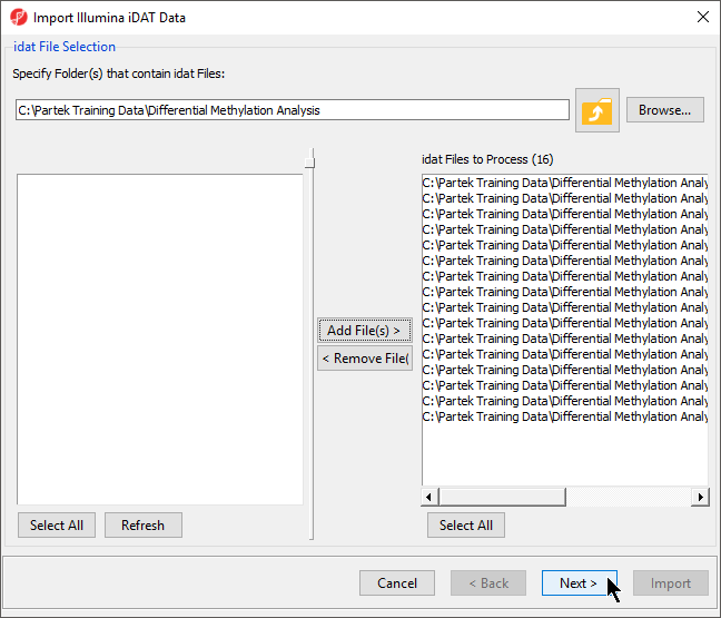
- Select Next >
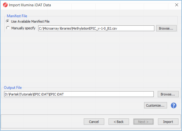
The following dialog (Figure 37) deals with the manifest file, i.e. probe annotation file. If a manifest file is not present locally, it will be downloaded in the Microarray libraries directory automatically. The download will take place in the background, with no particular message on the screen and it may take a few minutes, depending on the internet connection. If you have already downloaded the manifest file, to use it, select Use Available Manifest File option. If you have multiple versions available, you can pick an alternative by selecting Manually specify. The latter scenario corresponds to the situation where you In the future, you may want to reanalyze a data set at a later time. To enforce reproducibility, you may want to use using the same version of the manifest file that you used when the data was first processedduring the initial analysis, rather than downloading an up-to-date version.
To proceed with the tutorial, click Import. The result with be a spreadsheet with samples on rows (the initial identifier is the file name), probes on columns and beta values (normalised by functional normalisation) in the cells. Alternatively, if you wish to know more on what is happening during the import, go over the text below.
To facilitate this, the Manual specify option in the Manifest File section allows you to specify a specific version. For this tutorial, we will use the latest available manifest file.
| Numbered figure captions | |
|---|---|
|
...
...
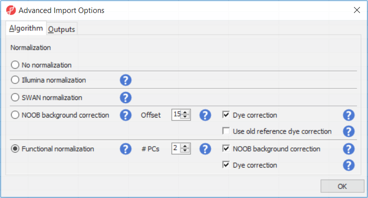
The Customize... button enables a granular control of the import process (Figure 4). First, the normalisation procedure is specified on the Algorithm tab (Figure 4).
Illumina normalisation is the algorithm implemented in GenomeStudio software and provides background subtraction and normalization to control probes. The results in Partek Genomics Suite may differ slightly from the GenomeStudio results, due to differences in selection of the control probes. SWAN normalization stands for subset-quantile within array normalization and was described in the manuscript by Maksimović et al.
Normal-exponential out-of-band (NOOB) background correction corresponds to the Noob background correction method, as implemented in Biocondutor's minfi package. Partek Genomics Suite uses the following options: offset = 15, dyeCorr = TRUE, dyeMethod= ”single” (in the other words, the preprocessFunnorm defaults).
Functional normalisation (default) is an extension of quantile normalisation, that uses control probes to remove the technical variation (Fortin J-P et al., Genome Biol 2014). Partek Genomics Suite uses the same defaults as the minfi package: nPCs = 2, sex = NULL, bgCorr = TRUE, dyeCorr = TRUE. The latter two options refer to the NOOB background correction. PC: principal components.
| Numbered figure captions | ||||
|---|---|---|---|---|
| ||||
|
| Numbered figure captions | ||||
|---|---|---|---|---|
| ||||
|
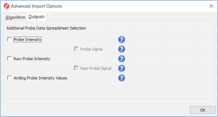
Probe Intensity results in a spreadsheet with samples on rows (with suffix _probe added to the file name), probes on columns, and the sum of raw methylated and unmethylated probe intensities in the cells (the spreadsheet name will also have suffix _probe). Upon selecting Probe Intensity, you can additionally select Probe Signal, which will append rows to the "probe intensity" spreadsheet: for each sample a row with methylated (suffix _meth) and a separate row with unmethylated (suffix _unmeth) intensities (in the other words, three rows per sample).
Raw Probe Intensity results in a spreadsheet with samples on rows (with suffix _raw added to the file name), probes on columns, and the sum of raw red and green probe intensities in the cells (the spreadsheet name will also have suffix _raw). Upon selecting Raw Probe Intensity, you can additionally select Raw Probe Signal, which will append rows to the "raw probe intensity" spreadseet: for each sample a row with red (suffix _red) and a separate row with green (suffix _green) intensities (in the other words, three rows per sample).
All the values discussed above will be log2 transformed upon import, and if you want to see the values in the linear space, select Antilog Probe Intensity Values.
...
| |||
|
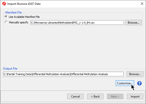
By default the output file destination is set to the file containing your .idat files and the name matches the file folder name. The name and location of the output file can be changed using the Output File panel.
- Select Customize to view advanced options for data normalization
In the Algorithm tab of the Advanced Import Options dialog (Figure 8), there are five options available. Select the (![]() ) next to each method for details. We recommend using the default options; however, advanced users can select their preferred normalization method. If you want to import probe intensity, raw probe intensity, probe signals, raw probe signals, or anti-log probe intensity values, they can be added to the data import using the Outputs tab of the Advanced Import Options dialog. Probe intensities and raw probe intensities can be used for advanced troubleshooting purposes and antiloged antilog probe intensities can be used for copy number detection. For this tutorial, we do not need to import any of these values.
) next to each method for details. We recommend using the default options; however, advanced users can select their preferred normalization method. If you want to import probe intensity, raw probe intensity, probe signals, raw probe signals, or anti-log probe intensity values, they can be added to the data import using the Outputs tab of the Advanced Import Options dialog. Probe intensities and raw probe intensities can be used for advanced troubleshooting purposes and antiloged antilog probe intensities can be used for copy number detection. For this tutorial, we do not need to import any of these values.
Section Heading
Section headings should use level 2 heading, while the content of the section should use paragraph (which is the default). You can choose the style in the first dropdown in toolbar.
| Numbered figure captions | ||||
|---|---|---|---|---|
| ||||
|

- Select OK to close the Advanced Import Options dialog
- Select Import on the Import Illumina iDAT data dialog
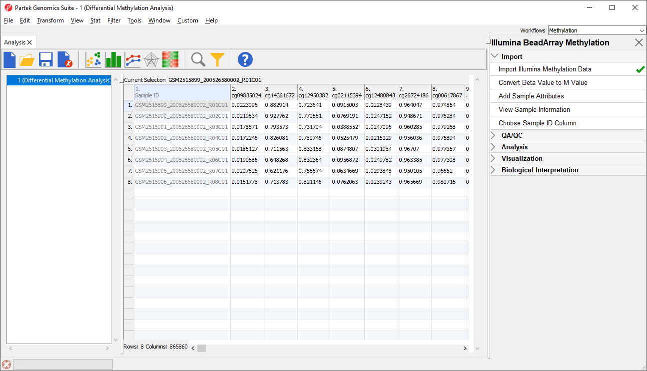
The imported and normalized data will appear as a spreadsheet 1 (Differential Methylation Analysis) (Figure 9)
| Numbered figure captions | ||||
|---|---|---|---|---|
| ||||
|
| Page Turner | ||
|---|---|---|
|
| Additional assistance |
|---|
|
| Rate Macro | ||
|---|---|---|
|
Overview
Content Tools