Page History
...
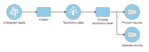
- Click a Taxonomic data node
- Choose Choose taxonomic level from the Metagenomic section of the toolbox
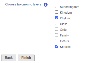
- Check one or more taxonomic levels. The options are Superkingdom, Kingdom, Phylum, Class, Order, Family, Genus, or Species (Figure 1). A separate output data node will be generated for each one that is selected (Figure 2)
- Click Finish
The choice of taxonomic level depends on which level you want to perform downstream analysis on and your research question. For example, if you want to know which families of bacteria are the most abundant in your sample, choose the family level. If you want to see which species are differentially abundant in different groups of samples, choose the species level.
| Numbered figure captions | ||||
|---|---|---|---|---|
| ||||
|
| Numbered figure captions | ||||
|---|---|---|---|---|
| ||||
|
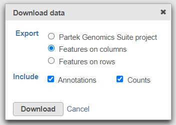
Download a count matrix
...
| Numbered figure captions | ||||
|---|---|---|---|---|
| ||||
|
| Numbered figure captions | ||||
|---|---|---|---|---|
| ||||
|
...
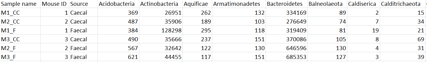
The taxon-level count data node(s) behave like any other count matrix in Partek Flow. This means you can perform most of the tasks you would normally perform on gene expression data. For example, you can normalize the species counts, perform principal components analysis (PCA), and use ANOVA to detect differentially abundant species in different groups of samples (Figure 5). Additional visualizations can also be generated including heatmaps, volcano plots, dot plots, and more.
...
Overview
Content Tools