Page History
...
| Numbered figure captions | ||||
|---|---|---|---|---|
| ||||
|
...
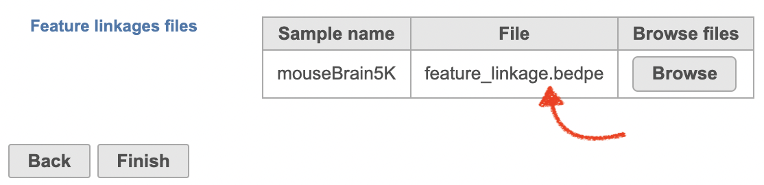
There will be no inputs needed if the FASTQ is converted to counts matrix within Flow. However, if users processed the FASTQ files outside of Partek, and imported the counts matrix into Flow later. The feature_linkage.bedpe file in outs/analysis/feature_linkage from Cell Ranger output will be needed for each sample (Figure 2) to complete the analysis.
| Numbered figure captions | ||||
|---|---|---|---|---|
| ||||
|
For data where no sample attributes are specified, the peak detection pairs need to be manually defined. In the example in Figure 1, there only two samples. Under the Define pairs section, the left panel lists all the sample names uploaded to the project (H3K27 and Mock). Add one pair at a time by dragging the corresponding samples to either the IP panel on the top-right or the Control panel on the bottom-right. If no control samples are present in the experiment, leave the Control panel blank. If more than one ChIP or Control samples are added, the samples will be combined (or pooled) during the analysis. After defining a pair, click the Add pair button.
...
Task report
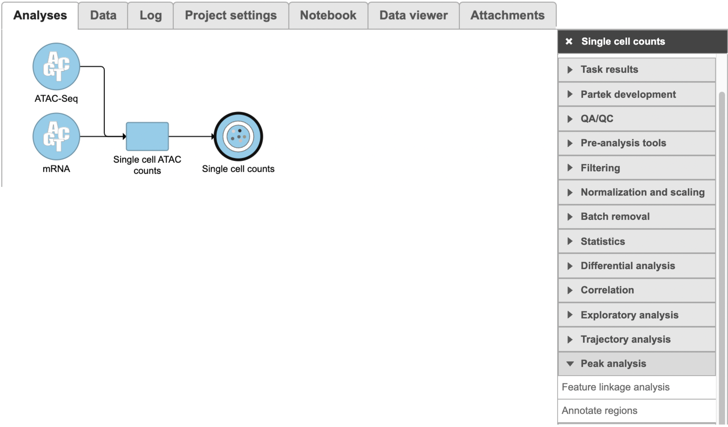
A new datanode will be displayed as the task is finished. Double click on the output datanode, Flow will bring you to the IGV browser where you could explore the “co-expressed”feature pairs (Figure 3).
| Numbered figure captions | ||||
|---|---|---|---|---|
| ||||
|

When running the MACS2 task, sample attributes will be used to define the multiple pairs (Figure 4). There is an IP-Input pair for each time point, so the Pair attribute is the Time attribute. The Control attribute is the attribute that differentiates between the Input and IP groups, and in this example, it is the ChIP attribute. Finally, the Control term is labeled as Input in the example.
| Numbered figure captions | ||||
|---|---|---|---|---|
| ||||
|

...
| Numbered figure captions | ||||
|---|---|---|---|---|
| ||||
|

If multiple pairs are added in the Pairs table, the peak detection is performed on each pair independently.
Peaks report
In the task report, each pair will generate a list of peaks displayed in a table (Figure 6). Use the drop down menu next to Peaks detected for... to select the pair.
| Numbered figure captions | ||||
|---|---|---|---|---|
| ||||
|

In the report table, each row is a region of a peak and includes the following information:
- Absolute summit: base pair location of peak summit
- Pileup: pileup height at peak summit
- -log10(pvalue): negative log10 pvalue for the peak summit
- Fold enrichment: fold enrichment for the peak summit against random Poisson distribution with local lambda
- -log10(qvalue): negative log10 qvalue at peak summit
- a peak name generated by the MACS2 algorithm
Click the browse to peak button () to invoke chromosome view and zoom into that location.
Click the Download button at the lower-right corner to download the peaks in a text file.
References
...
| |
|
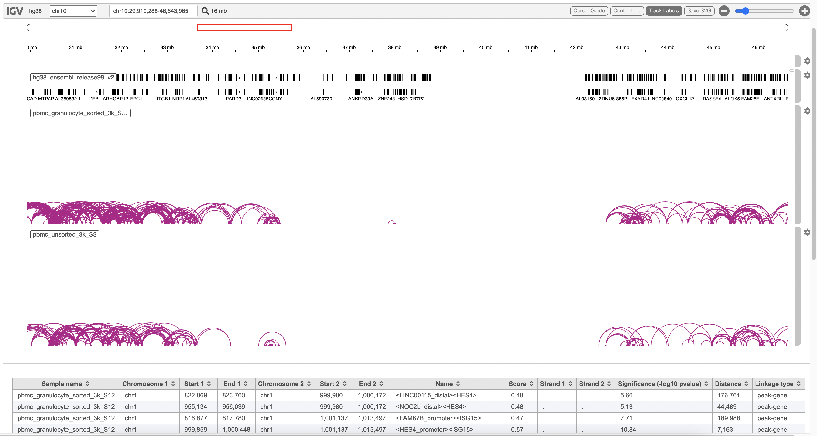
The feature_linkage.bedpe file[2] outputted from Cell Ranger pipeline is available in task report as a table. In the report table, each row is a region of a peak and includes the following information:
- Sample name: name for each sample
- Chromosome 1: the name of the chromosome on which the first feature exists.
- Start 1: the starting position of the first feature on that chromosome.
- End 1: the ending position of the first feature on that chromosome.
- Chromosome 2: the name of the chromosome on which the second feature exists.
- Start 2: the starting position of the second feature on that chromosome.
- End 2: the ending position of the second feature on that chromosome.
- Name: the name of the linkage features with the format of <name1><name2>, in which name1 and name2 are based on gene symbol or peak annotation.
- Score: linkage correlation, ranging from -1 to 1.
- Strand 1: all set to ".".
- Strand 2: all set to ".".
- Significance: linkage significance: -log10 (p-value) after multiple testing correction (FDR, false discovery rate). Capped at 299.
- Distance: distance in base pairs from feature 2 to feature 1.
- Linkage type: can be "peak-peak", "gene-peak" or "peak-gene" depending on the type of gene or peak for feature 1 and feature 2.
Filter feature linkage task
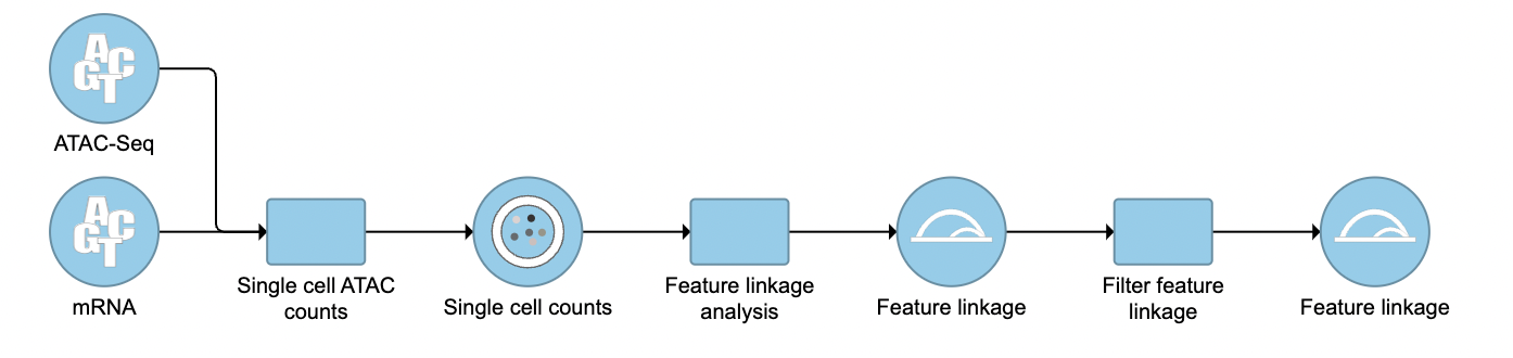
To filter out and visualize only the linkages that users are interested in is also made possible through the Filter feature linkages task in Flow (Figure 4). Users are able to download the .bedpe file from Flow and explore them via their stand-alone IGV.
| Numbered figure captions | ||||
|---|---|---|---|---|
| ||||
|
References
- https://software.broadinstitute.org/software/igv/
- https://support.10xgenomics.com/single-cell-multiome-atac-gex/software/pipelines/latest/output/analysis
| Additional assistance |
|---|
| Rate Macro | ||
|---|---|---|
|
...
Overview
Content Tools