Page History
...
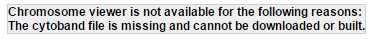
By default, the Chromosome view shows a cytoband track at the top of the canvas. If a cytoband file for your genome has not been added to Partek FlowPartek Flow, a warning will appear (Figure 301). In that case, go to the Library File Management page and download or create a cytoband file.
| Numbered figure captions | ||||
|---|---|---|---|---|
| ||||
|
The red box (Figure 312) indicates the part of the chromosome that is currently depicted on the canvas.
| Numbered figure captions | ||||
|---|---|---|---|---|
|
...
|

Reference Genome
The sequence of the reference genome is added to the Chromosome view by default, as long as it has been added to the respective genome on the Library File Management page. However, its presence (or absence) in the viewer depends on the current magnification. At low power, the track is hidden and you will see the message - Track hidden (zoom to view). At high power, on the other hand, the Reference genome track becomes visible (Figure 323) and is supplemented by the genomic coordinates (below the sequence). A vertical guide helps you to align the bases between Aligned reads and Reference genome tracks. Depending on the reference genome file, some bases may be shown in lowercase letters, symbolizing repetitive sequences, or other sequences masked by a tool such as RepeatMasker.
...
...
| Numbered figure captions | ||||
|---|---|---|---|---|
|
...
|

Variant Database
If a variant database file (such as dbSNP) for your genome is present on the Library File Management page, you will be able to include variant annotation track in your visualization (to add a variant database to the viewer, use the control panel on the right).
The variants will be shown adjacent to the Reference genome track (Figure 333). If the database contains no frequency information on alternative alleles, the alleles will be drawn as bars (an example is the SNP on the left in Figure 334). If the frequency information is available, the relative frequency of each variant will be represented by a column (the SNP on the right in Figure 334).
| Numbered figure captions | ||||
|---|---|---|---|---|
| ||||
|

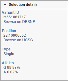
Note that the frequency information for each allele will be parsed out from the chosen database. That information can be retrieved by selecting a variant using the selection mode and will be shown in the Selection details section of the control panel. Using the example shown in Figure 334, the details of the left database variant can be seen in Figure 345. The most frequent allele at that locus is G (hence, yellow the yellow column is plotted above the Reference genome track), which matches the base call of the reference genome.
| Numbered figure captions | ||||
|---|---|---|---|---|
| ||||
|
If your variant database stores indels, they will be depicted using green (insertion) or red (deletion) symbols (Figure 356) pointing to deleted bases.
| Numbered figure captions | ||||
|---|---|---|---|---|
| ||||
|

Other Annotation Tracks
Additional annotation tracks can be added to the viewer with the help of the Select tracks dialog (Figure 14) as long as they have been associated with the genome you are working on in the Library File Management.
A common choice of an additional track is a transcript database, such as RefSeq (Figure 367). All the database entries are displayed, using common a common depiction of exons as boxes and introns as lines connecting them. Untranslated regions (UTRs) are seen as narrow boxes. The arrows indicate directionality.
| Numbered figure captions | ||||
|---|---|---|---|---|
| ||||
Customizing the View
Controls
Chromosome view can be customized by using the control panel on the left (Figure 37). The Attribute and Order By controls show options depending on the current project, while the content of the Annotate amino acids control depends on the annotation files associated with the current genome build in the Library File Management. In order for any change to take place, push the Apply button.
| Numbered figure captions | ||||
|---|---|---|---|---|
| ||||
Group data by
The first option, Group data by, specifies the number of Alignments tracks (Figure 38). All will result in only one track, with all the samples on it. Sample creates one track per sample, while Attribute produces one Alignments track per level of the Attribute (i.e. one track per group).
| Numbered figure captions | ||||
|---|---|---|---|---|
| ||||
All Sample Attribute |
Annotate amino acids by
Annotate amino acids by controls the appearance of the Amino acids track and allows you to pick the transcript database that will be used to plot codons (Figure 39). The drop down list shows the databases currently available for the selected genome (additional databases can be added via Library File Management).
| Numbered figure captions | ||||
|---|---|---|---|---|
| ||||
Color by
Color by option affects the colouring of the Alignments track and Isoform proportion track. When Sample is selected from the drop-down list, individual samples will be shown on the aforementioned tracks, each sample being given a different colour. If attributes were assigned to samples, they will also be visible in the Color by drop-down (Figure 40) and you will be able to highlight levels of the selected attribute (Figure 41).
| Numbered figure captions | ||||
|---|---|---|---|---|
| ||||
| Numbered figure captions | ||||
|---|---|---|---|---|
| ||||
Color by Sample Color by <Attribute> |
The effect of the option to Color by Base can be seen with high power magnification (Figure 42). Individual base calls are highlighted by different colours. When that option is chosen at low power magnification, all the bases are shown in grey.
| Numbered figure captions | ||||
|---|---|---|---|---|
| ||||
Finally, Color by Match can be used to quickly identify mismatches against the reference genome. A matching base is coloured in blue, while mismatch bases are shown in yellow.
Read histogram Y-axis scales
The maximum of the y-axis of Alignments tracks is set by Read histogram Y axis scales option (Figure 43). When using Independent, the y-axis for each track is set individually, based on the maximum within that sample. On the other hand, Linked uses the maximum across all the samples and uses that value as the maximum for all.
| Numbered figure captions | ||||
|---|---|---|---|---|
| ||||
Independent Linked |
Read histogram type
Read histogram type changes the presentation of the Alignments track and should be used in conjunction with the Group data by and Color by tracks to get the desired visualisation.
...
| Numbered figure captions | ||||
|---|---|---|---|---|
| ||||
To show average coverage per locus, switch Read histogram type to Average and leave Color by as is (i.e. by group) (Figure 45). With this setting, Chromosome view will calculate the average by dividing the total coverage per locus by the number of samples. Note that using Color by Sample would not make sense here. Although Figure 44 looks quite like Figure 43, the y-axis range is different.
| Numbered figure captions | ||||
|---|---|---|---|---|
| ||||
Finally, the option Overlay is useful if you want to directly compare base counts over several samples (or groups) as each will be represented by a line (i.e. no stacking). Example in Figure 46 is based on microarray data, showing three groups on the same Alignments track. The red group has the highest base counts, while the counts in the blue group are much lower.
| Numbered figure captions | ||||
|---|---|---|---|---|
| ||||
Transcript label
...
| Numbered figure captions | ||||
|---|---|---|---|---|
| ||||
Transcript label: Gene Transcript label: Transcript |
Reads pileup and probe color
| Numbered figure captions | ||||
|---|---|---|---|---|
| ||||
Reads pileup color: Strand Reads pileup color: Base |
Probe color control customizes the appearance of Probe intensities track (Figure 49). When set to Intensity, colour of a probe reflects its intensity, using a colour gradient from white (low) to admiral (high). Alternatively, when Strand is turned on, probes on the reverse strand are in parakeet green, while probe on the forward strand are in sky blue.
| Numbered figure captions | ||||
|---|---|---|---|---|
| ||||
Probe color: Intensity |
If a variant database is available for the current genome, the variants can be added to the Reference genome track (Figure 33). To show the variants, point the Variant database control to the database of your choice.
...
| Numbered figure captions | ||||
|---|---|---|---|---|
| ||||
Track Order
The position of the tracks on canvas can be controlled by using the Track order tool. If you want a track to be visible all the time, i.e. while scrolling up or down, pin it to the top or to the bottom. Figure 51 shows Cytoband track pinnned to the top of the canvas and Reference genome track pinned to the bottom of the canvas. To unpin a track, click on the pin icon ( ). The track will be unpinned and a message No tracks are pinnned to the top / bottom will appear. To pin a track, drag the track name to the No tracks… message. Alternatively, you can use the green arrows (
) to pin a track. When you mouse over an arrow, the new position of the track will be highlighted on the canvas; click on the arrow to accept.
A track can be hidden (meaning it will not be visible) by selecting the red minus, or unhidden by selecting the green plus icon.
...
| Numbered figure captions | ||||
|---|---|---|---|---|
| ||||
Selection Details
At the bottom of the control panel you will find the Selection details section (Figure 52). It is used to display information on the element selected on the canvas (using the Pointer mode).
| Numbered figure captions | ||||
|---|---|---|---|---|
| ||||
| Additional assistance |
|---|
|
|
| Additional assistance |
|---|
| Page Turner | ||
|---|---|---|
|
| Rate Macro | ||
|---|---|---|
|
Overview
Content Tools