Page History
...
| Numbered figure captions | ||||
|---|---|---|---|---|
| ||||
|
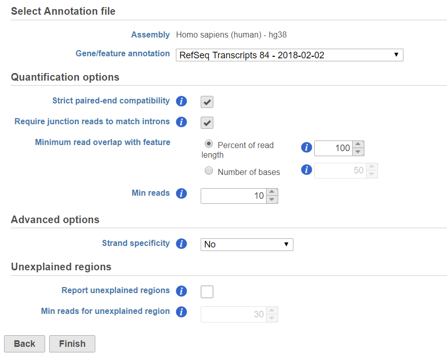
If the bam file is imported, you need to select the assembly with which the reads were aligned to, and which annotation model file you will use to quantify from the drop-down menus (Figure 2).
...
If the Require junction reads to match introns check button is selected, only junction reads that overlap with exonic regions and match the skipped bases of an intron in the transcript will be included in the calculation. Otherwise, as long as the reads overlap within the exonic region, they will be counted. Detailed information about read compatibility can be found in the Understanding Reads white paper.
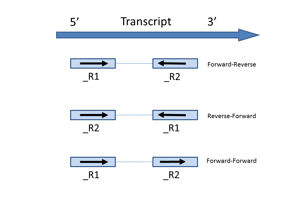
Some library preparations reverse transcribe the mRNA into double stranded cDNA, thus losing strand information. In this case, the total transcript count will include all the reads that map to a transcript location. Others will preserve the strand information of the original transcript by only synthesizing the first strand cDNA. Thus, only the reads that have sense compatibility with the transcripts will be included in the calculation. We recommend verifying with the data source how the NGS library was prepared to ensure correct option selection.
...
| Numbered figure captions | ||||
|---|---|---|---|---|
| ||||
|
Minimum read overlap with feature can be specified in percentage of read length or number of bases. By default, a read has to be 100% within a feature. You can allow some overhanging bases outside the exonic region by modifying these parameters.
Min reads optioin option is a filter, by default only the features whose sum of the reads across all samples that are greater than or equal to 10 will be reported. To report all the features in the annotation file, set the value to 0.
...
In the annotation file, there might be multiple features in the same location, or one read might have multiple alignments, so the read count of a feature might not be an integer. Our white paper on the Partek E/M algorithm has more details on Partek’s implementation the E/M algorithm initially described by Xing et al. [1]
...
| Numbered figure captions | ||||
|---|---|---|---|---|
| ||||
|
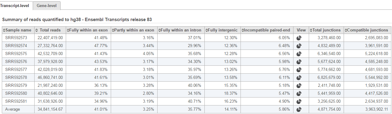
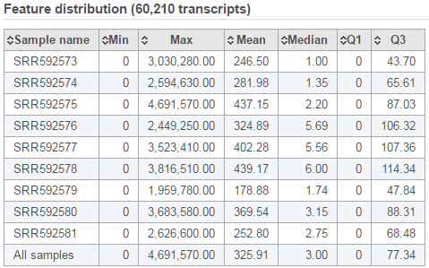
The second table contains feature distribution information on each sample and across all the samples, number of features in the annotation model is displayed on the table title (Figure 5).
...
| Numbered figure captions | ||||
|---|---|---|---|---|
| ||||
|
The bar chart displaying the distribution of raw read counts is helpful in assessing the expression level distribution within each sample. The X-axis is the read count range, Y axis is the number of features within the range, each bar is a sample. Hovering your mouse over the bar displays the following information (Figure 6):
...
| Numbered figure captions | ||||
|---|---|---|---|---|
| ||||
|

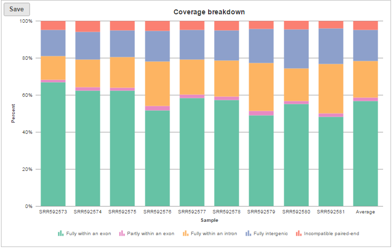
The coverage breakdown bar chart is a graphical representation of the reads summary table for each sample (Figure 7)
...
| Numbered figure captions | ||||
|---|---|---|---|---|
| ||||
|
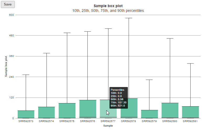
In the box-whisker plot, each box is a sample on X-axis, the box represents 25th and 75th percentile, the whiskers represent 10th and 90th percentile, Y-axis represents the read counts, when you hover over each box, detailed sample information is displayed (Figure 8).
| Numbered figure captions | ||||
|---|---|---|---|---|
| ||||
|
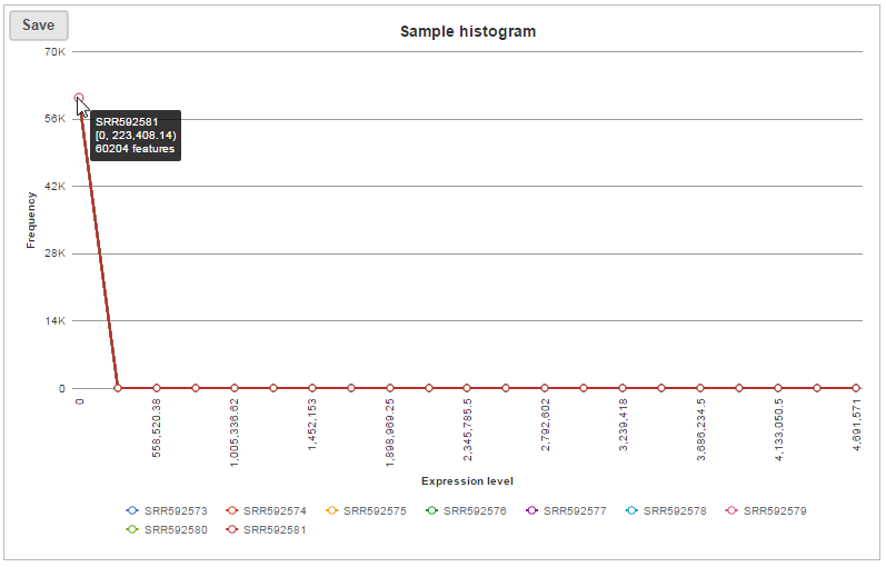
In sample histogram, each line represents a sample and the range of read counts are divided into 20 bins. Clicking on a sample in the legend will hide the line for that specific sample. Hovering over each circle displays detailed information about the sample and that specific bin (Figure 9). The information includes:
...
| Numbered figure captions | ||||
|---|---|---|---|---|
| ||||
|
The box whisker and sample histogram plots are helpful for understanding the expression level distribution across samples. This may indicate that normalization between samples might be needed prior to downstream analysis. Note that all four visualizations are disabled for results with more than 30 samples.
...
Overview
Content Tools