Join us for a webinar: The complexities of spatial multiomics unraveled
May 2
Page History
...
| Numbered figure captions | ||||
|---|---|---|---|---|
| ||||
|
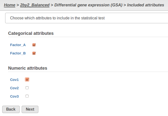
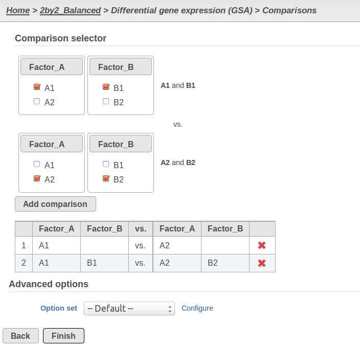
Currently, GSA is capable of considering the following five response distributions: Normal, Lognormal, Lognormal with shrinkage, Negative Binomial, Poisson (Figure 1). The GSA interface has an option to restrict this pool of distributions in any way, e.g. by specifying just one response distribution. The user also specifies the factors that may enter the model (Figure 2A) and comparisons for categorical factors (Figure 2B).
...
| Numbered figure captions | ||||
|---|---|---|---|---|
| ||||
A) Choosing factors (attributes) in GSA
B) Choosing comparisons in GSA |
...
| Numbered figure captions | ||||
|---|---|---|---|---|
| ||||
|
Obtaining reproducible results in GSA
...
| Numbered figure captions | ||||
|---|---|---|---|---|
| ||||
|
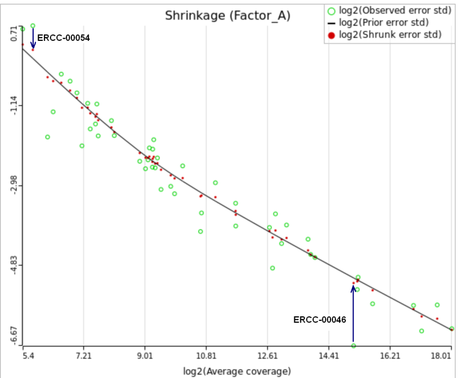
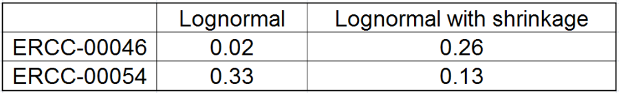
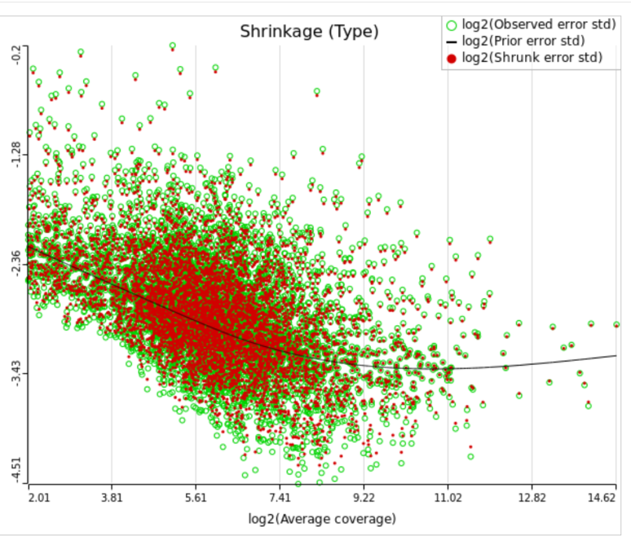
All other things being equal, the comparison p-value goes up as the magnitude of error term goes up, and vice-versa. As a result, the "shrunken" p-value goes up (down) if the error term is adjusted up (down). Table 1 reports some results for two features highlighted in Figure 4
...
| Numbered figure captions | ||||
|---|---|---|---|---|
| ||||
|
For a large sample size, the amount of shrinkage is small, (Figure 5), and the "Lognormal" and "Lognormal with shrinkage" p-values become virtually identical.
...
| Numbered figure captions | ||||
|---|---|---|---|---|
| ||||
|
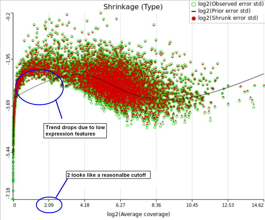
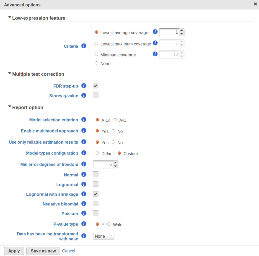
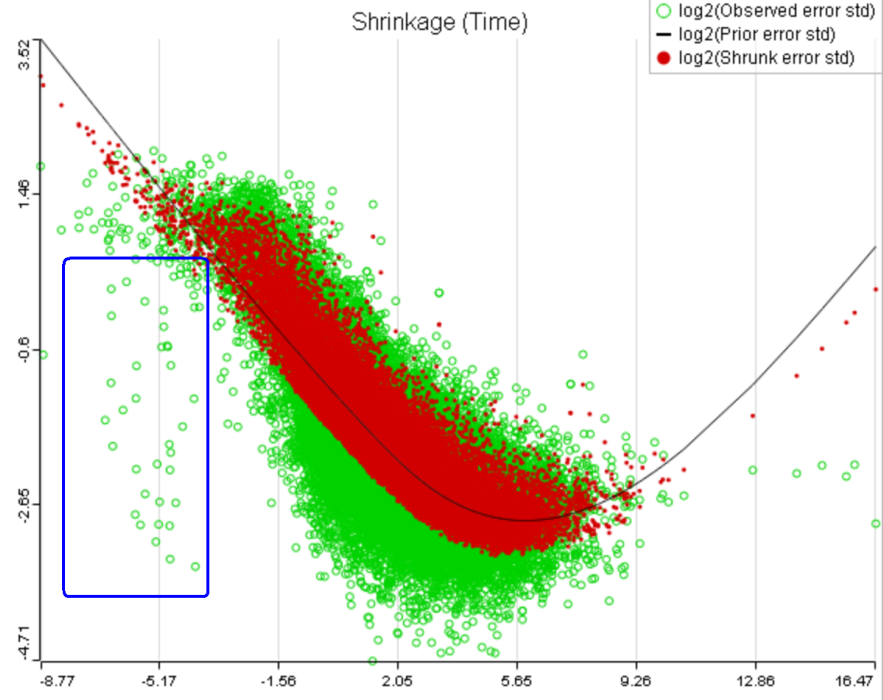
One important usage of the shrinkage plot is a meaningful setting of low expression threshold in Low expression filter section (Figure 6). For features with low expression, the proportion of zero counts is high. Such features are less likely to be of interest in the study, and, in any case, they cannot be modeled well by a continuous distribution, such as Lognormal. Note that adding a positive offset to get rid of zeros does not help because that does not affect the error term of a lognormal model much. A high proportion of zeros can ultimately result in a drop in the trend in the leftmost part of the shrinkage plot (Figure 56).
A rule of thumb suggested by limma authors is to set the low expression threshold to get rid of the drop and to obtain a monotone decreasing trend in the left-hand part of the plot.
...
| Numbered figure captions | ||||
|---|---|---|---|---|
| ||||
|
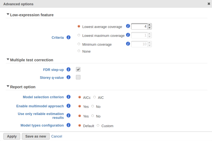
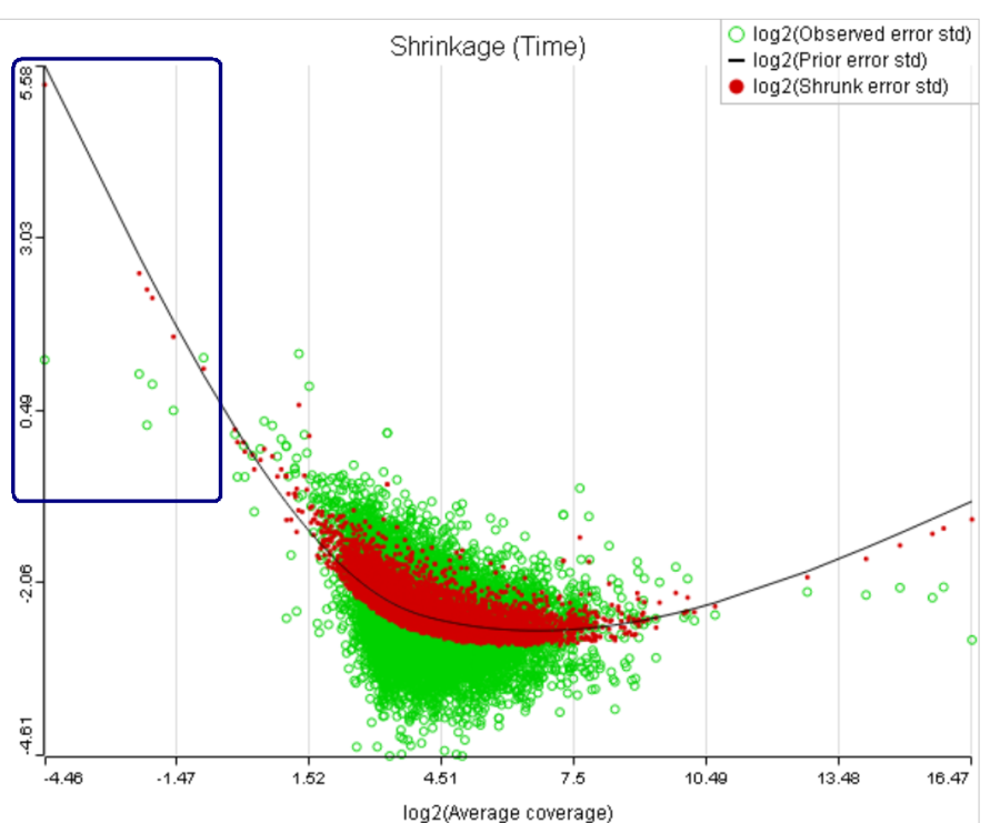
For instance, in Figure 5 it looks like a threshold of 2 can get us what we want. Since the x axis is on the log2 scale, the corresponding value for "Lowest average coverage" is 222^2=4 (Figure 6). After we set the filter that way and rerun GSA, the shrinkage plots takes the required form (Figure 7).
...
| Numbered figure captions | ||||
|---|---|---|---|---|
| ||||
|
Note that it is possible to achieve a similar effect by increasing a threshold of "Lowest maximal coverage", "Minimum coverage", or any similar filtering option (Figure 6). However, using "Average coverage" is the most straightforward: the shrinkage procedure uses log2(Average coverage) as an independent variable to fit the trend, so the x axis in the shrinkage plot is always log2(Average coverage) regardless of the filtering option chosen in Figure 6.
...
| Numbered figure captions | ||||
|---|---|---|---|---|
| ||||
A) Average expression threshold can be raised to get rid of low expression features with abnormal error terms, circled in blue
B) Six low expression features (circled in blue) account for a very sharp increase in the trend which can have an unduly large effect on overall results |
...
| Numbered figure captions | ||||
|---|---|---|---|---|
| ||||
|
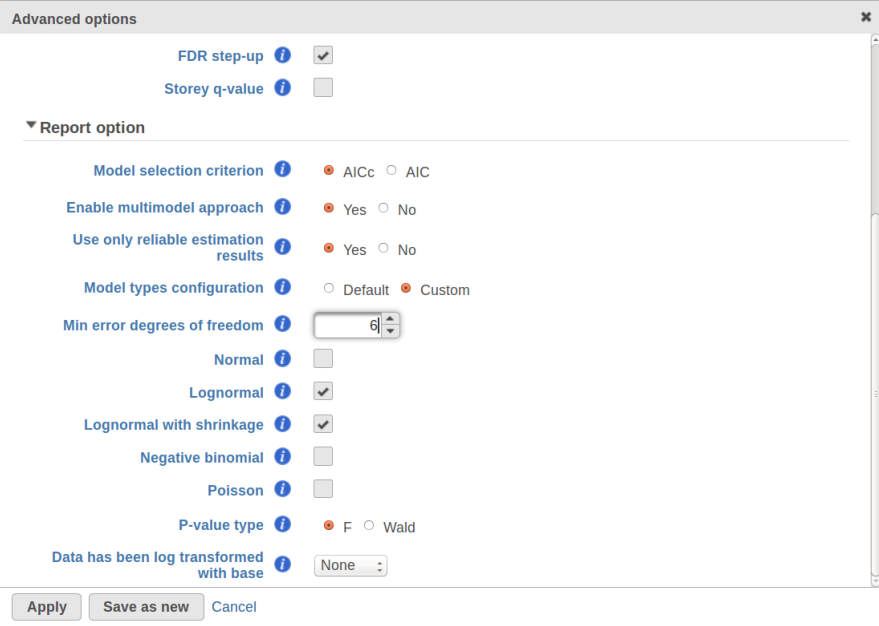
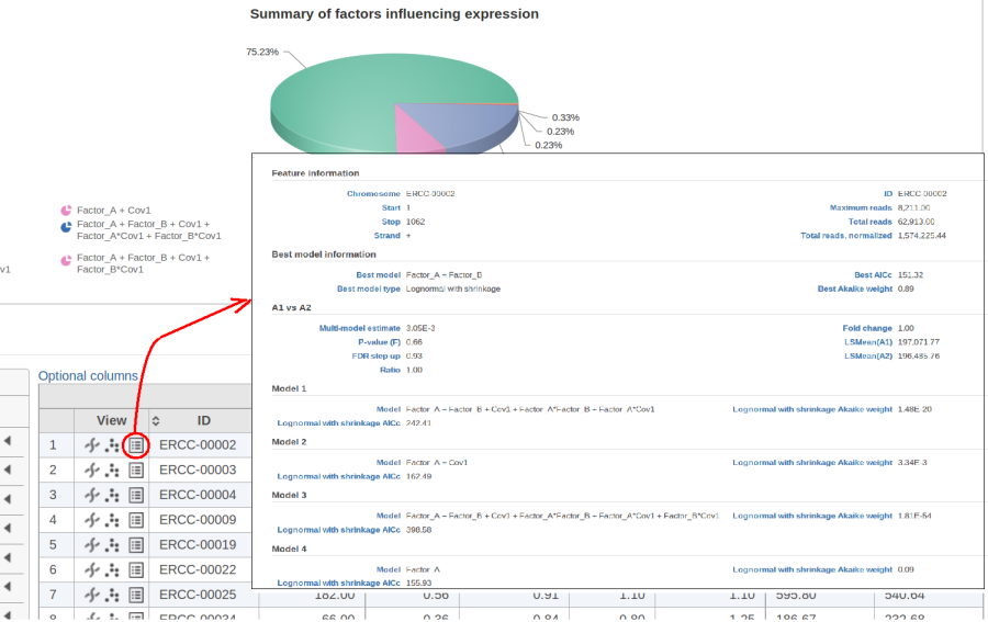
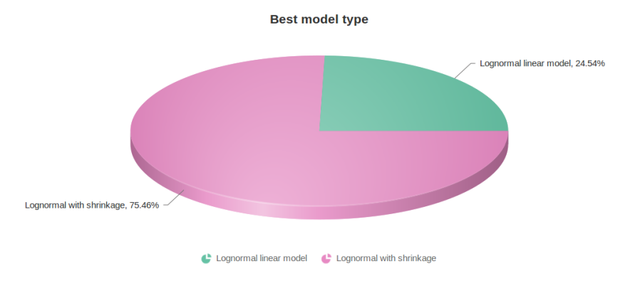
Figure 10 contains a pie chart for the dataset whose shrinkage plot is displayed in Figure 4. Because of a small sample size (two groups with four observations each) we see that, overall, shrinkage is beneficial: for an "average" feature, Akaike weight for feature-specific Lognormal is 25%, whereas Lognormal with shrinkage weighs 75%.
...
| Numbered figure captions | ||||
|---|---|---|---|---|
| ||||
|
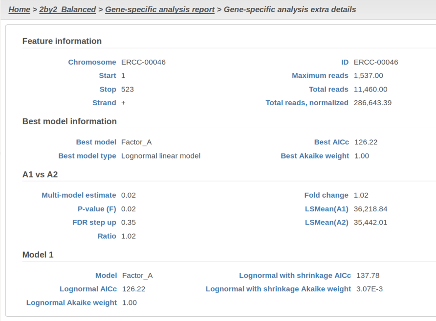
At the same time, if we look at ERCC-00046 specifically (Figure 11) we see that Lognormal with shrinkage fits so bad that its Akaike weight is virtually zero, despite having fewer parameters than feature-specific Lognormal.
...
| Numbered figure captions | ||||
|---|---|---|---|---|
| ||||
|
Using multimodel inference appears to be a better alternative to the ad hoc method in DESeq2 that switches shrinkage on and off all the way. Once again, it is both technically possible and emotionally tempting to automate the handling of abnormal features by enabling both Lognormal models in GSA and applying them to all of the transcripts. Unfortunately, that can make the results less reproducible overall, even though it is likely to yield more accurate conclusions about the drastically outlying features.
...
Overview
Content Tools