Page History
...
| Numbered figure captions | ||||
|---|---|---|---|---|
| ||||
|
The format of the output is the same as the input data format, the node is called Normalized counts. This data node can be selected and normalized further using the same task.
Selecting Methods
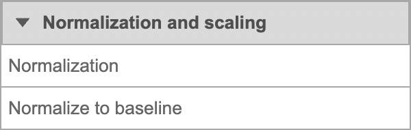
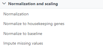
Select whether you want your data normalized on a per sample or per feature basis (Figure 2). Some transformations are performed on each value independently of others e.g. log transformation, and you will get an identical result regardless of your choice.
...
Note that each task can only perform normalization on samples or features. If you wish to perform both transformations, run two normalization tasks successively. To normalize the data, click on a method from the left panel, then drag and drop the method to the right panel. Add all normalization methods you wish to perform. Alternatively, you can click on the green plus button () on each method to add it. Multiple methods can be added to the right panel and they will be processed in the order they are listed. You can change the order of methods by dragging each method up or down. To remove a method from the Normalization order panel, click the minus button (
![]() ) to the right of the method. Click Finish, when you are done choosing the normalization methods you have chosen.
) to the right of the method. Click Finish, when you are done choosing the normalization methods you have chosen.
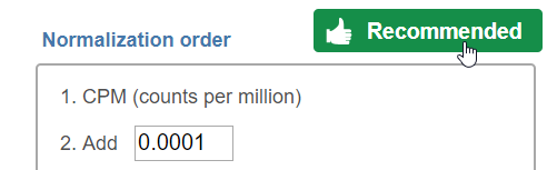
Recommended Methods
For some data nodes, recommended methods are available:
...
| Numbered figure captions | ||||
|---|---|---|---|---|
| ||||
|
Normalization Methods
Below is the notation that will be used to explain each method:
...
- Remove all the features that have 0 reads in all samples.
- Calculate the effective library size per sample: effective library size = (raw library size (in millions))*((upper quartile for a particular sample)/ (geometric mean of upper quartiles in all the samples))
- Get the normalized counts by dividing the raw counts per feature by the effective library size (for the respective sample)
Normalization Report
The Normalization report includes the Normalization methods used, a Feature distribution table, Box-whisker plots of the Expression signal before and after normalization, and Sample histogram charts before and after normalization. Note that all visualizations are disabled for results with more than 30 samples.
Normalization methods
A summary of the normalization methods performed. They are listed by the order they were performed.
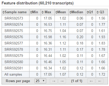
Feature distribution table
A table that presents descriptive statistics on each sample, the last row is the grand statistics across all samples (Figure 4).
...
| Numbered figure captions | ||||
|---|---|---|---|---|
| ||||
|
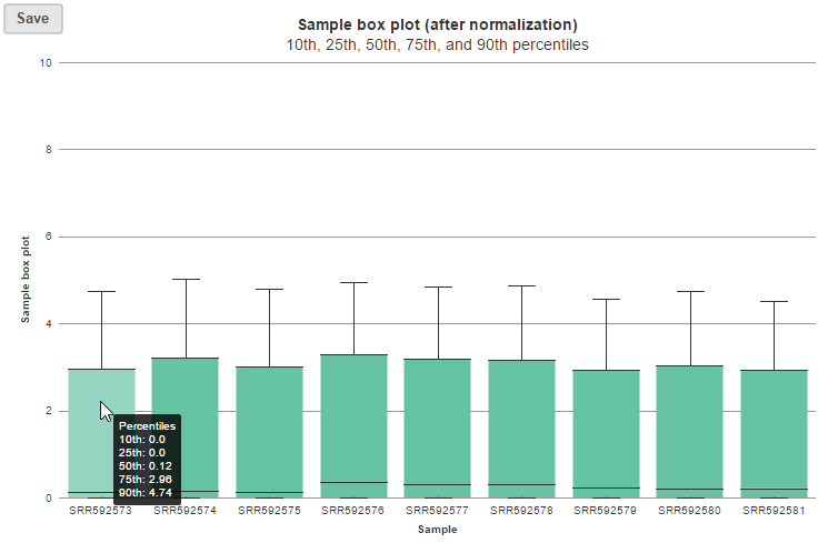
Expression signal
These box-whisker plots show the expression signal distribution for each sample before and after normalization. When you mouse over on each bar in the plot, a balloon would show detailed percentile information (Figure 5).
...
| Numbered figure captions | ||||
|---|---|---|---|---|
| ||||
|
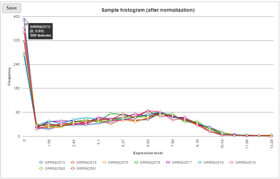
Sample histogram
A histogram is displayed for data before and after it is normalized. Each line is a sample, where the X axis is the range of the data in the node and the Y-axis is the frequency of the value within the range. When you mouse over a circle which represent a center of an interval, detailed information will appear in a balloon (Figure 6). It includes:
...
| Numbered figure captions | ||||
|---|---|---|---|---|
| ||||
|
References
- Bolstad BM, Irizarry RA, Astrand M, Speed, TP. A Comparison of Normalization Methods for High Density Oligonucleotide Array Data Based on Bias and Variance. Bioinformatics. 2003; 19(2): 185-193.
- Mortazavi A, Williams BA, McCue K, Schaeffer L, Wold B. Mapping and quantifying mammalian transcriptomes by RNA-Seq. Nat Methods. 2008; 5(7): 621–628.
- Bullard JH, Purdom E, Hansen KD, Dudoit S. Evaluation of statistical methods for normalization and differential expression in mRNA-Seq experiments. BMC Bioinformatics. 2010; 11: 94.
- Robinson MD, Oshlack A. A scaling normalization method for differential expression analysis of RNA-seq data. Genome Biol. 2010; 11: R25.
- Dillies MA, Rau A, Aubert J et al. A comprehensive evaluation of normalization methods for Illumina high-throughput RNA sequencing data analysis. Brief Bioinform. 2013; 14(6): 671-83.
- Wagner GP, Kin K, Lynch VJ. Measurement of mRNA abundance using RNA-seq data. Theory Biosci. 2012; 131(4): 281-5.
- Ritchie ME, Phipson B, Wu D et al. Limma powers differential expression analyses for RNA-sequencing and microarray studies. Nucleic Acids Res. 2015; 43(15):e97.
...
Overview
Content Tools