Page History
To detect differential methylation between CpG loci in different experimental groups, we can perform an ANOVA test. For this tutorial, we will perform a simple one-way ANOVA to compare naive-state hPSCs treated with shRNAs targeting NANOG to those targeting POU5F1.
- Select Defect Differential Methylation from the Analysis section of the Illumina BeadArray Methylation workflow
- Select 2. State and3. shRNA treatment from the Experimental Factor(s) panel by holding the Ctrl key on your keyboard and selecting both itemspanel
- Select Add Factor > to move 2. State and3. shRNA treatment to the ANOVA Factor(s) panel Select Add Interaction > to add the interaction between 2. State and 3. shRNA treatment (Figure 1)
| Numbered figure captions | ||||
|---|---|---|---|---|
| ||||
|
- Select Contrasts...
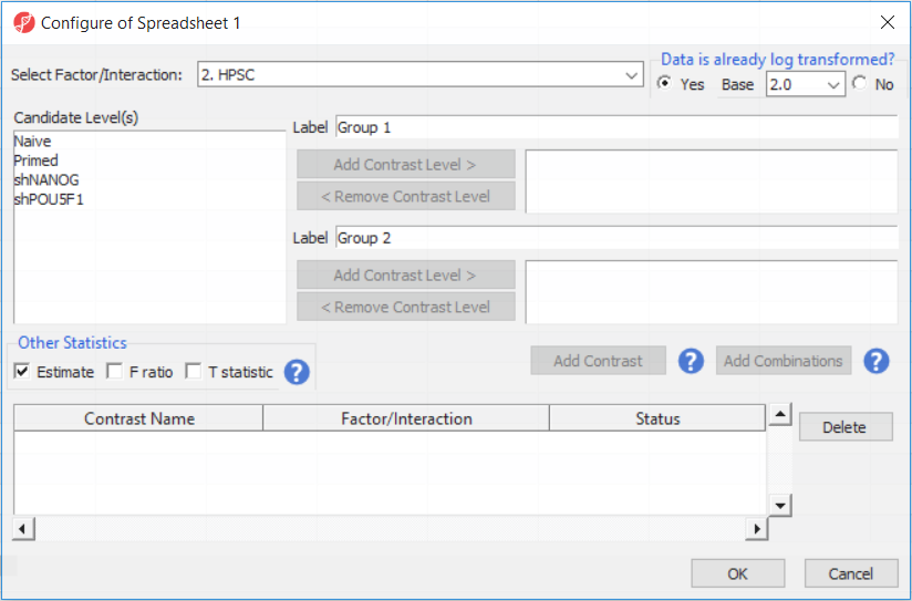
- Select Yes for Data is already log transformed?
- Select 2. State * 3. shRNA treatment from the Select Factor/Interaction drop-down menu
- Select all four options in the Candidate Level(s) panel by selecting each while holding the Ctrl key on your keyboard
- Select because M-values are based on logit transformation
- Select shPOU5F1
- Select Add Contrast Level > for Group 1 to add shPOU5F1 to Group 1, which will be renamed shPOU5F1
- Repeat steps to add all four options shNANOG to Group 2
- Select Add Combination
- Select OK to close the Configuration dialog
- Select OK to close the ANOVA dialog and run the ANOVA
...
- 2
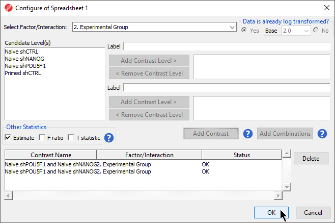
- Select the Estimate box in the Other Statistics section of the Configure dialog (Figure 2)
By default, the fold-change value for each contrast and, in addition to that, if you want to will be calculated. Selecting Estimate will also include the difference in methylation levels between the groups at each CpG site in the output, check the Estimate box in the Other Statistics section of the dialog (Figure 2). The setup of the contrasts has implications on downstream steps, in particular on filtering the . These values will be needed later in the tutorial when we filter the differentially methylated loci.
...
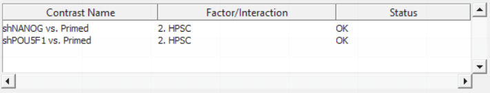
For this exercise, we shall compare primed HPSC with suppression of OCT4 (shPOU5F1) and primed HPSC with suppression of NANOG (shNANOG) with the baseline primed cells. To start with, select the Primed group in the Candidate Level(s) box and push Add Contrast Level > to move the Primed group to Group 2 (lower box). Then Ctrl & select both shPOU5F1 and shNANOG in the Candidate Level(s) box and push Add Contrast Level > to move them to Group 1 (upper box). Then click Add Combinations and confirm that two contrast have been created as seen in Figure 3.
| Numbered figure captions | ||||
|---|---|---|---|---|
| ||||
|
Push OK to confirm the contrast (and close the contrast dialog) and again to start the ANOVA calculation.
| Numbered figure captions | |
|---|---|
|
...
| |||
|
- Select Add Combination
- Select OK to close the Configuration dialog
- Select OK to close the ANOVA dialog and run the ANOVA
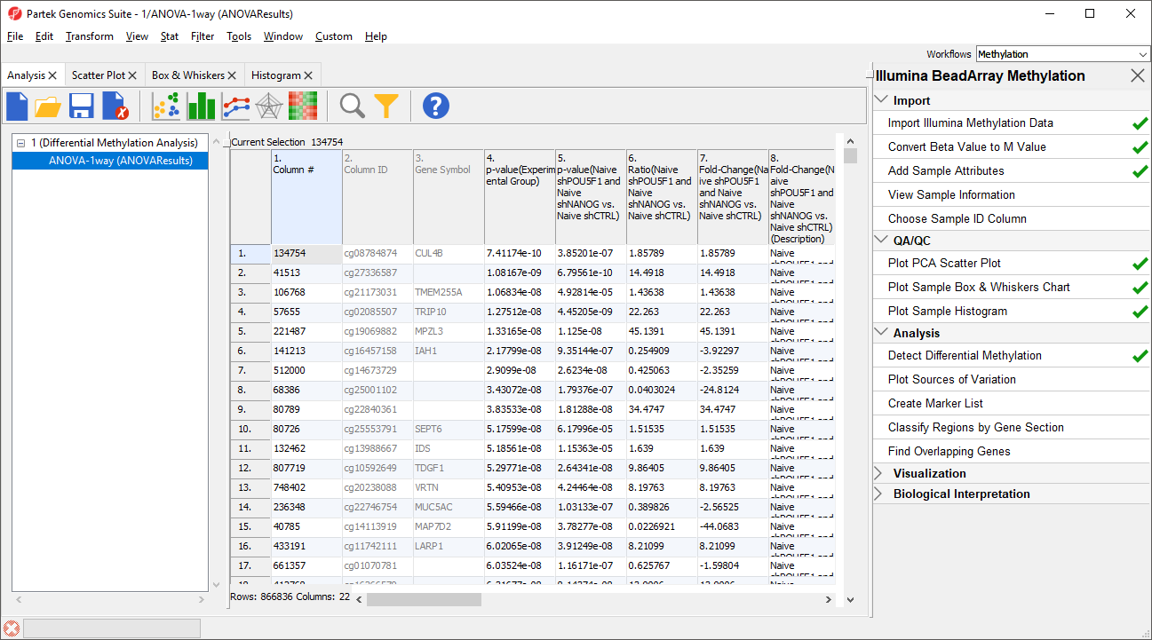
The results will appear as ANOVA-1way (ANOVAResults), a child spreadsheet of 1 (Differential Methylation Analysis). Each row of the spreadsheet represents a single CpG locus (identified by Column ID).
The first time you use MethylationEPIC array, the manifest file needs to be configured and the window like the one in Figure 4 will pop up. First select the second option (Chromosome is in one column and the physical location is in another column). Marker ID is on the first column (Ilmn ID), Chromosome is on the column CHR, while the Physical Position is on the MAPINFO column. Set according to Figure 4 and select Close. This enable Partek Genomics Suite to parse out probe annotation from the manifest file.
...
Overview
Content Tools