An RNA-Seq quantification algorithm determines how aligned reads are assigned (i.e. mapped) to the transcript model. In turn, the quantification result provides a basis for the expression estimation and novel transcript discovery.
Each combination of sequencing instrument and sequencing protocol varies in terms of how precisely it is able to estimate the transcript abundance, and/or what data biases it propagates downstream. A good quantification algorithm is expected to extract the maximal amount of information from the reads, and, importantly, to adjust for the biases of the sequencer and protocol. However, the practical impact of biases depends on the purpose of the study. Likewise, if the study agenda includes some particular items such as novel transcript discovery, this alone can determine the choice of a combination of aligner and quantification package.
Challenges and Solutions
The most recognized quantification issues common to RNA-Seq include the following:
- Multireads (multimappers)
- Sequence (composition) bias
- Position bias
- GC bias
Multireads
Multireads (or multimappers) are reads aligning to multiple locations in the genome. Three different approaches to handling those reads have been described.
- Disallowing multireads (obsolete) (1, 2).
- Full expectation-maximization (EM) algorithm (3), as implemented in Partek® Flow®, with slight modifications.
- The “rescue” method implemented in Cufflinks (4 - 7), which is equivalent to the first (presumably the most informative) iteration of EM.
For paired-end reads with multiple alignments, it is possible to improve quantification by extracting information from the fragment (insert) size distribution. This feature is available in Cufflinks.
Sequence Bias
Sequence bias refers to the observation that the reads that have particular subsequences of nucleotides (typically, at 5’ or 3’ end) may be over- or underrepresented due to some artifacts of sequencing technology (8, 9) (for an illustration see Figure 2 in Roberts et al. (4)). The corresponding bias correction is implemented in Cufflinks.
Position Bias
Position bias (10 - 12) is manifested in unequal distribution of reads along the length of a transcript (see Figure 4 in Jiang et al. (12)). The corresponding correction is implemented in Cufflinks.
GC Bias
GC bias means that the estimated abundance of a transcript (gene) is dependent on its GC content. While Dohm et al. reported that GC-rich regions attract reads (see Figure 2 in (13)), another study argued that the dependence can go either way (see Figure 2 in Zheng et al. (14)). Although there is no available package that contains the GC bias correction Cufflinks team shown that in some cases the GC bias is highly correlated with the sequence bias and then a separate GC correction is unnecessary.
Assessing the Practical Impact of Biases
An accepted way to measure the impact of a certain bias is as follows: take a number of transcripts (genes) and perform the quantification with and without bias correction and then observe the change in concordance between the expected (known) and the estimated abundance. Initially, the expected abundances were estimated based on qPCR (4). More recently, the usage of presumably more accurate External RNA Controls Consortium (ERCC) controls took hold (12, 15). In the latter approach, the known abundance is measured as concentration of transcripts in attomoles/μL.
The estimated abundance is derived from fragments per kilobase of transcript per million aligned reads (FPKM)/reads per kilobase of transcript per million aligned reads (RPKM) values delivered by the quantification algorithm. The concordance between known and estimated abundances is measured by the r2, a value ranging from 0% to 100%, where 100% corresponds to perfect estimation of abundance.
The studies of Roberts et al. (4) and Li et al. (10) measured the importance of sequence and position bias correction based on qPCR using a set of genes from Microarray Quality Control project (MAQC). Roberts and colleagues reported that, when both sequence and position bias are accounted for, the r2 goes up by about 5%, from 75.3% to 80.7%. The impact of position bias is reported to be small relative to that of sequence bias.
Li and Dewey (10) showed that RSEM quantification package, that implements only the position bias correction, delivers the r2 of 69%. For comparison, running Cufflinks on the same dataset with the position bias correction obtained the r2 of only 71%. When both sequence and position bias corrections were enabled in Cufflinks, the r2 went up to 79%. We can conclude that, for real datasets, the impact of position bias is negligible, and the impact of sequence bias is about 5-8%.
More qPCR-based insight was given by Li et al. (9). They proposed a so-called MART model for the sequence bias, which was subsequently incorporated in Cufflinks in May 2011. According to their finding, the sequence bias correction has a negligible effect on the estimated abundance. However, this conclusion changes when they conditioned on the gene length and fold change: long genes were not affected by sequencing bias as much as short genes, and the impact was sizable for the genes with the largest fold change.
The results of a ERCC-based study of Jiang (12), who used a dataset consisting of 4.4 billion 76-bases paired-end reads with 96 ERCC transcripts. They found that, while the sequencing bias does exist on short genomic intervals, it disappeared (averaged out) very quickly as the length of transcript (gene) increased. They also found some evidence of GC content and length biases. The length bias was not covered earlier in Challenges and Solutions (at the beginning of this document) because length is a feature of the entire transcript (gene), and therefore it can be adjusted for downstream of quantification, as proposed in (16). A similar approach can be applied to GC bias, and it should work as long as our goal is to compare the abundances of the same transcript (gene) under different conditions.
On the other hand, suppose we want to compare the expression of two isoforms that differ by a short subsequence, such as a 50 bp exon. Then, the GC bias can be practically significant because the difference in expression may be attributed to the exon’s GC content. Likewise, it may be attributed to the nucleotide composition of the exon that causes it to attract an unfair number of reads due to the sequence bias. In that case, the GC and sequence biases need to be adjusted for during quantification.
Partek EM Algorithm: Validation of Quantification Results
Data from the Sequencing Quality Control Project (SEQC) was obtained from the Mayo Clinic site, which used the Illumina HiSeq2000. The dataset consists of about one billion of 2×100 paired-end reads, which amounts to about 512 GB of uncompressed fastq files, with about 4 GB for each of the 128 samples.
To control the sequencing quality, 92 ERCC transcripts were used. The expected abundance (concentration) of the transcripts was known and it differed by a factor of one million across transcripts. The transcript reads come from two groups, Mix A and Mix B. The mixes were prepared in a way that, for each transcript, we knew the fold change between Mix A and Mix B (the fold change could take four distinct values). Therefore, we were able test the accuracy of both abundance and fold change estimation.
After Bowtie alignment to the ERCC reference file and filtering on base and alignment quality, about 2.3% of the original one billion reads were retained. For technical reasons, the reads were treated as single-end.
A drawback of ERCC transcripts is that they do not produce multireads, so it was impossible to compare all of the different approaches to multiread handling described above. Likewise, ERCC transcripts are not alternatively spliced, i.e. they do not contain a large number of isoforms that differ by a short exon. Therefore, we were not likely to observe the effect of sequencing bias and GC bias corrections.
Quantification was performed by Partek Flow with the EM algorithm and the plots of estimated vs. expected transcript abundance for Mix A and Mix B are in Figures 1 and 2 (respectively). As we can see, the r2 is about 97% and, hence, there is very little room for improvement in abundance estimation.
Furthermore, a fold change plot is given (Figure 3), comparing the estimated and expected fold change in Mix A vs. Mix B, for the four groups of transcripts with the known fold change values. The fold change values were calculated based on log2 transformed RPKM values for each transcript (control).
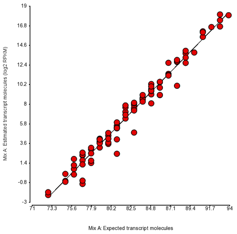
Figure 1. Comparison of expected number of molecules of ERCC Mix A and the estimated number of transcript molecules (log2 of RPKM values), obtained by Partek’s modification of expectation-maximization algorithm. Each dot is an ERCC control. r^2 = 0.97, regression y = 0.98 * x - 74.41
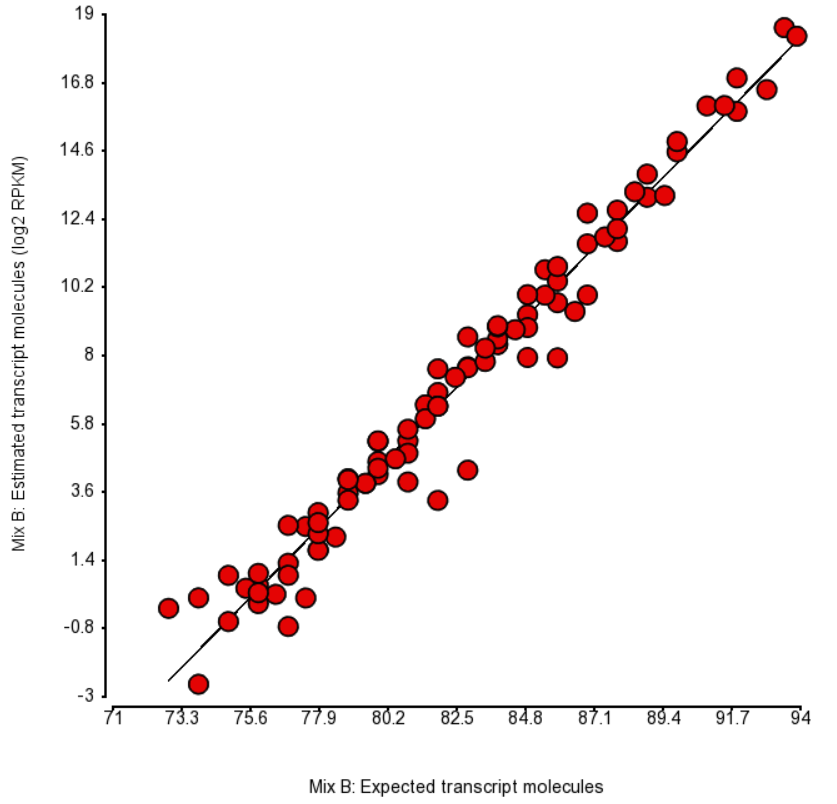
Figure 2. Comparison of expected number of molecules of ERCC Mix B and the estimated number of transcript molecules (log2 of RPKM values), obtained by Partek’s modification of expectation-maximization algorithm. Each dot is an ERCC control. r^2 = 0.97, regression y = 0.98 * x - 74.06
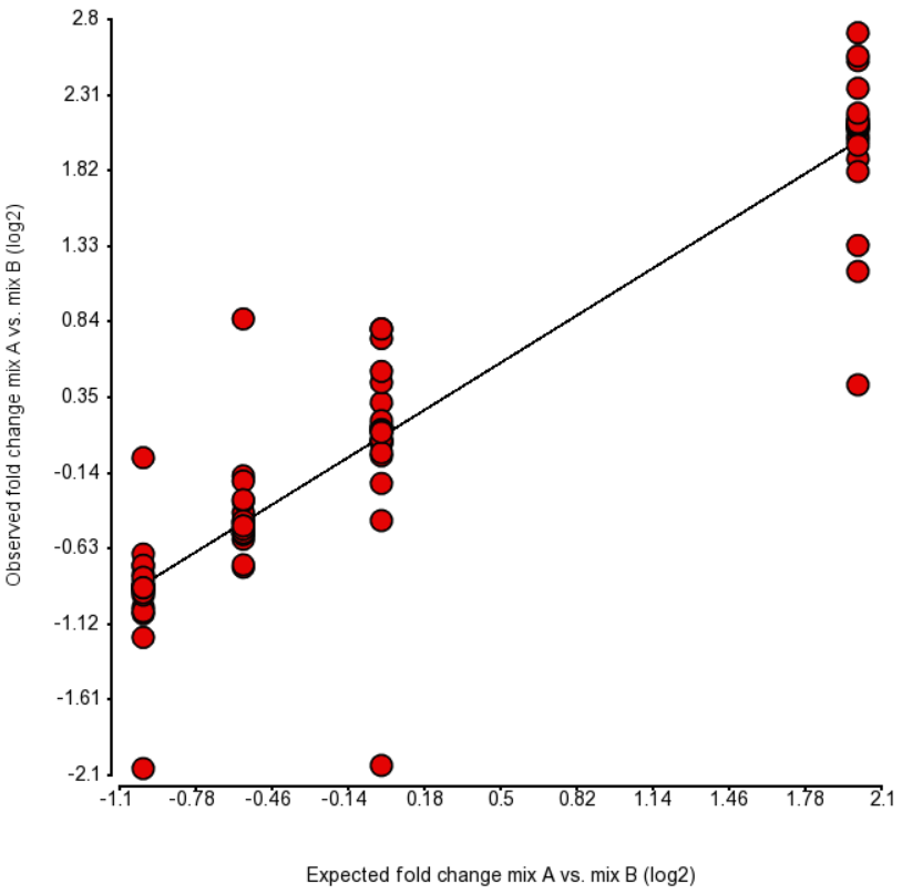
Figure 3. Comparison of expected fold change (log2) vs. observed fold change (log2) in ERCC Mix A vs. Mix B, for the four groups of transcripts with the known fold change values. Each dot is an ERCC control. r^2 = 0.87, regression y = 0.96 * x + 0.09
To test for possible biases in abundance estimates, we combined the approaches of Li et al. (9) and Jiang et al. (12). That amounted to regressing the estimated abundance not only on the expected abundance, but also on the transcript length, GC content, and the expected fold change, subjecting all the variables to log2 transformation.
We started with the full model containing four covariates and performed model selection based on two criteria: adjusted r2 (computed for all possible models) and stepwise regression (with a cutoff p-value of 0.15). The combined approach allowed us to consider both practical and statistical significance of the covariates.
The full model for Mix A (Table 1) has the highest adjusted r2, but it was only 0.01% better than the model consisting of the expected abundance and length only. The latter was also pointed to by the stepwise selection, so we nominated it as the best model (Table 2). While the length effect in the best model was statistically significant, the adjusted r2 was only 0.44% higher than that of the benchmark model (Table 3). Therefore, we found little evidence of the practical significance of the length bias.
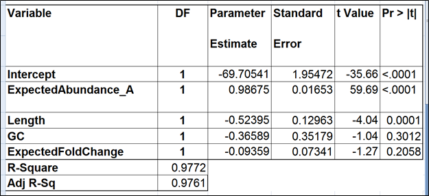 Table 1. Regression of the observed transcript abundance on the expected transcript abundance, transcript length, GC content, and the expected fold change, subjecting all the variables to log2 transformation. We started with the full model containing four covariates and performed model selection based on two criteria: adjusted r^2 (computed for all possible models) and stepwise regression (with a cutoff p-value of 0.15). The assessment was performed on the Mix A of ERCC, using Partek’s modified expectation-maximization (EM) algorithm for transcript quantification.
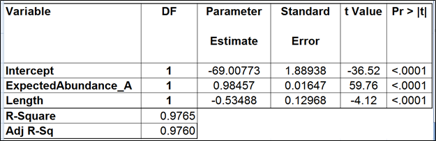 Table 2. Regression of the observed transcript abundance on the expected transcript abundance and transcript length (the best model). We started with the full model containing four covariates and performed model selection based on two criteria: adjusted r^2 (computed for all possible models) and stepwise regression (with a cutoff p-value of 0.15). The assessment was performed on the Mix A of ERCC, using Partek’s modified expectation-maximization (EM) algorithm for transcript quantification.
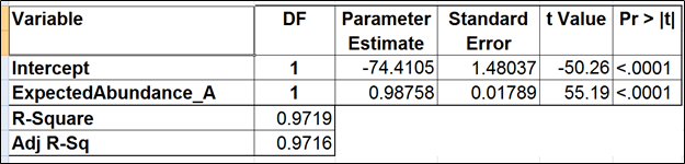 Table 3. Regression of the observed transcript abundance on the expected transcript abundance (the benchmark model). We started with the full model containing four covariates and performed model selection based on two criteria: adjusted r^2 (computed for all possible models) and stepwise regression (with a cutoff p-value of 0.15). The assessment was performed on the Mix A of ERCC, using Partek’s modified expectation-maximization (EM) algorithm for transcript quantification.
The full and the best models for the Mix B are shown in Tables 4 and 5 (respectively). Apparently, the regression failed to find evidence of any kind of bias.
Table 3. Regression of the observed transcript abundance on the expected transcript abundance (the benchmark model). We started with the full model containing four covariates and performed model selection based on two criteria: adjusted r^2 (computed for all possible models) and stepwise regression (with a cutoff p-value of 0.15). The assessment was performed on the Mix A of ERCC, using Partek’s modified expectation-maximization (EM) algorithm for transcript quantification.
The full and the best models for the Mix B are shown in Tables 4 and 5 (respectively). Apparently, the regression failed to find evidence of any kind of bias.
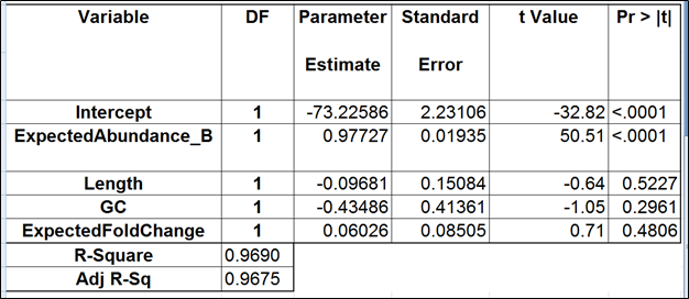 Table 4. Regression of the observed transcript abundance on the expected transcript abundance, transcript length, GC content, and the expected fold change, subjecting all the variables to log2 transformation. We started with the full model containing four covariates and performed model selection based on two criteria: adjusted r^2 (computed for all possible models) and stepwise regression (with a cutoff p-value of 0.15). The assessment was performed on the Mix B of ERCC, using Partek’s modified expectation-maximization (EM) algorithm for transcript quantification.
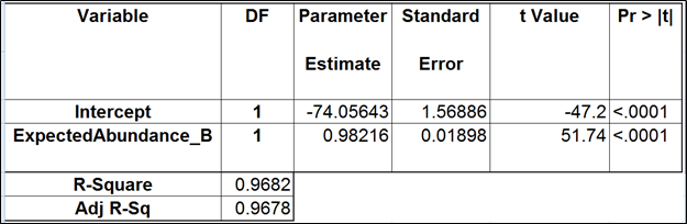 Table 5. Regression of the observed transcript abundance on the expected transcript abundance (the best model). We started with the full model containing four covariates and performed model selection based on two criteria: adjusted R2 (computed for all possible models) and stepwise regression (with a cutoff p-value of 0.15). The assessment was performed on the Mix A of ERCC, using Partek’s modified expectation-maximization (EM) algorithm for transcript quantification.
Conclusions
Although we did not report the results obtained by Cufflinks quantification algorithm, we believe that no extra analysis is necessary. First, the nature of ERCC approach does not make it a tool sensitive enough to detect the subtle effects that are estimated by Cufflinks quantification algorithm. Second, we showed that, even if those effects were taken into account, there would be very little room for improvement that could be detected by ERCC tools.
Jiang and colleagues came to a similar conclusion (12). Although they did not include the dose response and fold change plots in their manuscript, in personal correspondence they acknowledged that they had actually constructed the plots but failed to see a significant impact of the bias corrections implemented in Cufflinks. The minimal ERCC transcript length is about 250 bp, and, unless one interested in comparing isoforms that differ by a much shorter sequence (50 bp is a good estimate), the bias corrections are of little use.
References
Langmead B, Hansen KD, Leek JT. Cloud-scale RNA-sequencing differential expression analysis with Myrna. Genome Biol. 2010;11(8):R83.
Li J, Jiang H, Wong WH. Modeling non-uniformity in short-read rates in RNA-Seq data. Genome Biol. 2010;11:R50.
Xing Y, Yu T, Wu YN, Roy M, Kim J, Lee C. An expectation-maximization algorithm for probabilistic reconstructions of full-length isoforms from splice graphs. Nucleic Acids Res. 2006;34:3150-3160.
Roberts A, Trapnell C, Donaghey J, Rinn JL, Pachter L. Improving RNA-Seq expression estimates by correcting for fragment bias. Genome Biol. 2011;12:R22.
Trapnell C, Williams BA, Pertea G, et al. Transcript assembly and quantification by RNA-Seq reveals unannotated transcripts and isoform switching during cell differentiation. Nat Biotechnol. 2010;28:511-515.
Trapnell C, Roberts A, Goff L, et al. Differential gene and transcript expression analysis of RNA-seq experiments with TopHat and Cufflinks. Nat Protoc. 2012;7:562-578.
Roberts A, Pimentel H, Trapnell C, Pachter L. Identification of novel transcripts in annotated genomes using RNA-Seq. Bioinformatics. 2011;27:2325-2329.
Hansen KD, Brenner SE, Dudoit S. Biases in Illumina transcriptome sequencing caused by random hexamer priming. Nucleic Acids Res. 2010;38:e131.
Li J, Jiang H, Wong WH. Modeling non-uniformity in short-read rates in RNA-Seq data. Genome Biol. 2010;11:R50.
Li B, Ruotti V, Stewart RM, Thomson JA, Dewey CN. RNA-Seq gene expression estimation with read mapping uncertainty. Bioinformatics. 2010;26:493-500.
Leng N, Dawson JA, Thomson JA, et al. EBSeq: an empirical Bayes hierarchical model for inference in RNA-seq experiments. Bioinformatics. 2013;29:1035-1043.
Jiang L, Schlesinger F, Davis CA, et al. Synthetic spike-in standards for RNA-seq experiments. Genome Res. 2011;21:1543-1551.
Dohm JC, Lottaz C, Borodina T, Himmelbauer H. Substantial biases in ultra-short read data sets from high-throughput DNA sequencing. Nucleic Acids Res. 2008;36:e105.
Zheng W, Chung LM, Zhao H. Bias detection and correction in RNA-Sequencing data. BMC Bioinformatics. 2011;12:290.
ERCC RNA spike-in control mixes. http://tools.thermofisher.com/content/sfs/manuals/cms_086340.pdf Accessed: March 25, 2016
Oshlack A, Wakefield MJ. Transcript length bias in RNA-seq data confounds systems biology. Biol Direct. 2009;4:14.
Additional Assistance
If you need additional assistance, please visit our support page to submit a help ticket or find phone numbers for regional support.


| Your Rating: |
|
Results: |

|
38 | rates |
Overview
Content Tools
1 Comment
Melissa del Rosario
author: ilukic