Join us for a webinar: The complexities of spatial multiomics unraveled
May 2
Page History
...
| Numbered figure captions | ||||
|---|---|---|---|---|
| ||||
|
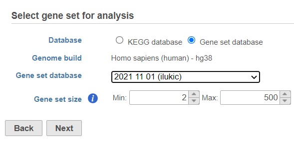
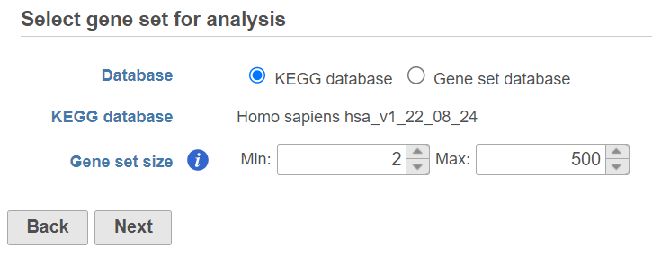
Once your choices are made, push Next to proceed.
...
| Numbered figure captions | ||||
|---|---|---|---|---|
| ||||
|
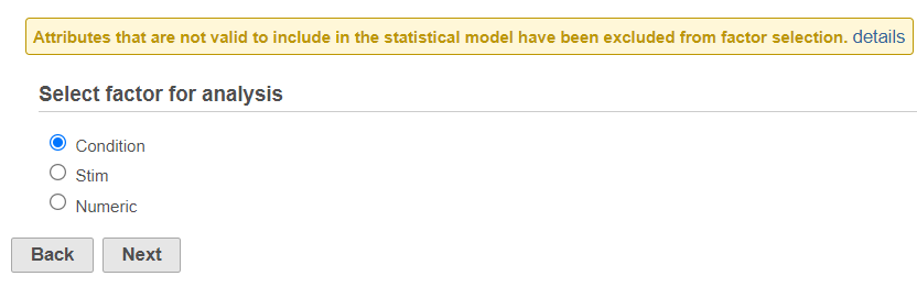
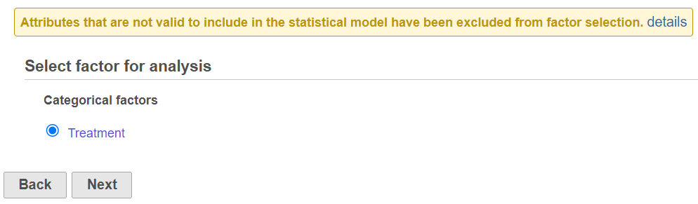
If the warning message is displayed, click on the details link to learn more about unavailable factors (an example is shown in Figure 5).
...
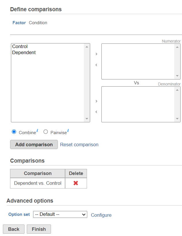
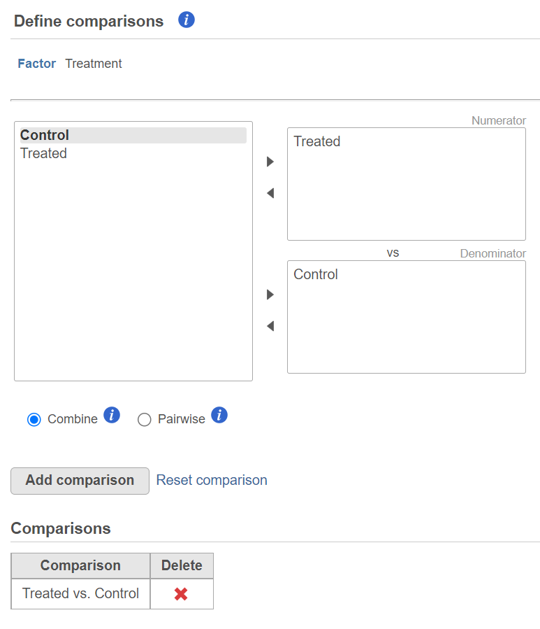
The third dialog is Define comparisons (Figure 6). The box on the left side displays the categories of the selected factor (shown as Factor). Use the arrow buttons (>) to move one of the factors to the Denominator box (that factor should be interpreted as the reference category) and the other factor to the Numerator box. Confirm your selection by pushing the Add comparison button and the comparison will be added to the Comparisons table (Figure 6).
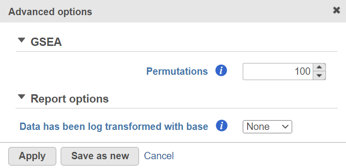
Low value filter is turned on by default and will remove all the genes with the lowest average coverage of 1.0 or below; if a filter feature task was performed before this task, the default low-value filter is set to None (for details please see the GSA chapter) .
| Numbered figure captions | ||||
|---|---|---|---|---|
| ||||
|
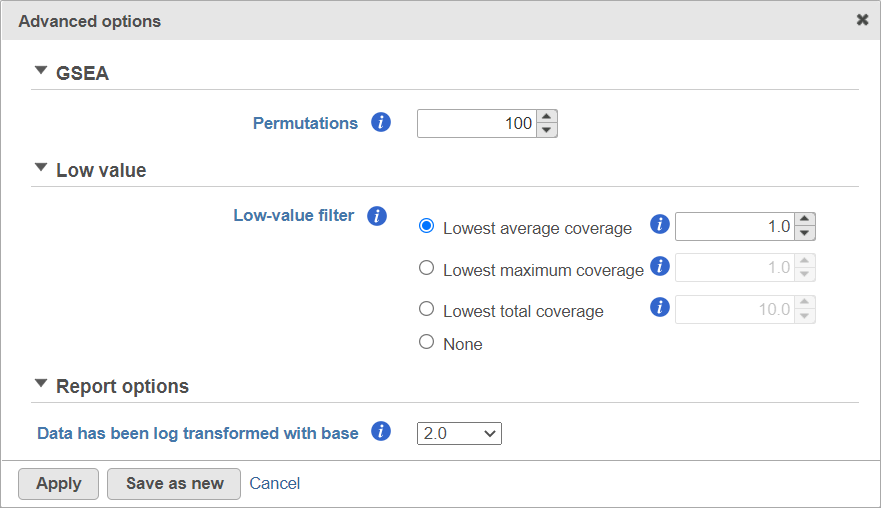
Push Finish to launch GSEA with the default settings.
Alternatively, click on the Configure icon to access the advanced options (Figure 7). Number of data permutations (needed to calculate the normalised enrichment scores) can be controlled using the Permutations option. Permutation is to randomly permute the group assignment across a given gene. For each permutation, a random order is computed, that order is used to compute the score for each gene. Low value filter is turned on by default and will remove all the genes with the lowest average coverage of 1.0 or below; if a filter feature task was performed before this task, the default low-value filter is set to None (for details please see the GSA chapter) . Finally, if you start your project by importing a count matrix (i.e. as opposed to generating the count matrix using Partek Flow), you need to specify whether the expression values were log transformed before the import (use the Data has been log transformed with base drop down).
...
| Numbered figure captions | ||||
|---|---|---|---|---|
| ||||
|
GSEA Results
When the task completes, double click on the GSEA task node (Figure 8) to view the report.
...
| Numbered figure captions | ||||
|---|---|---|---|---|
| ||||
|
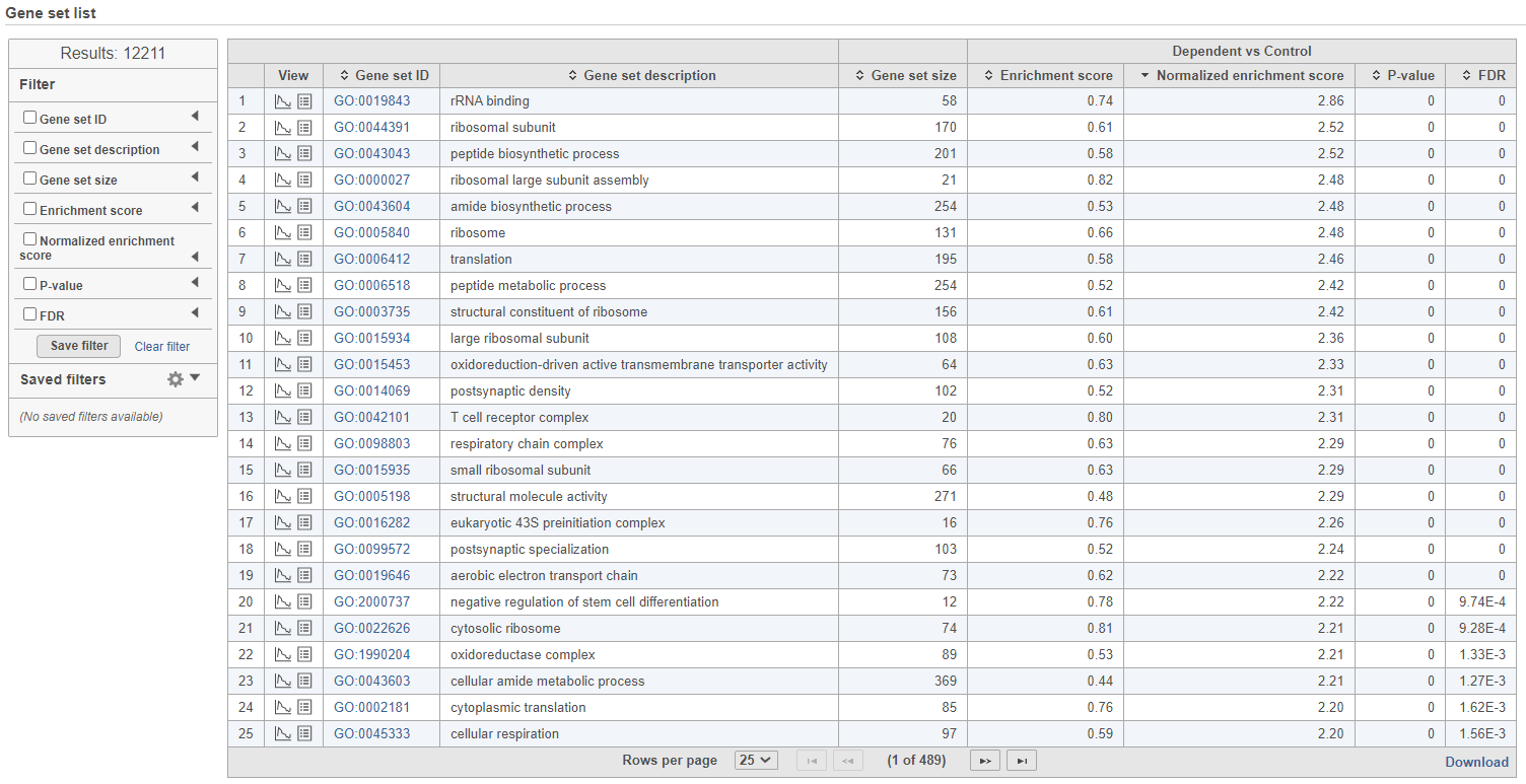
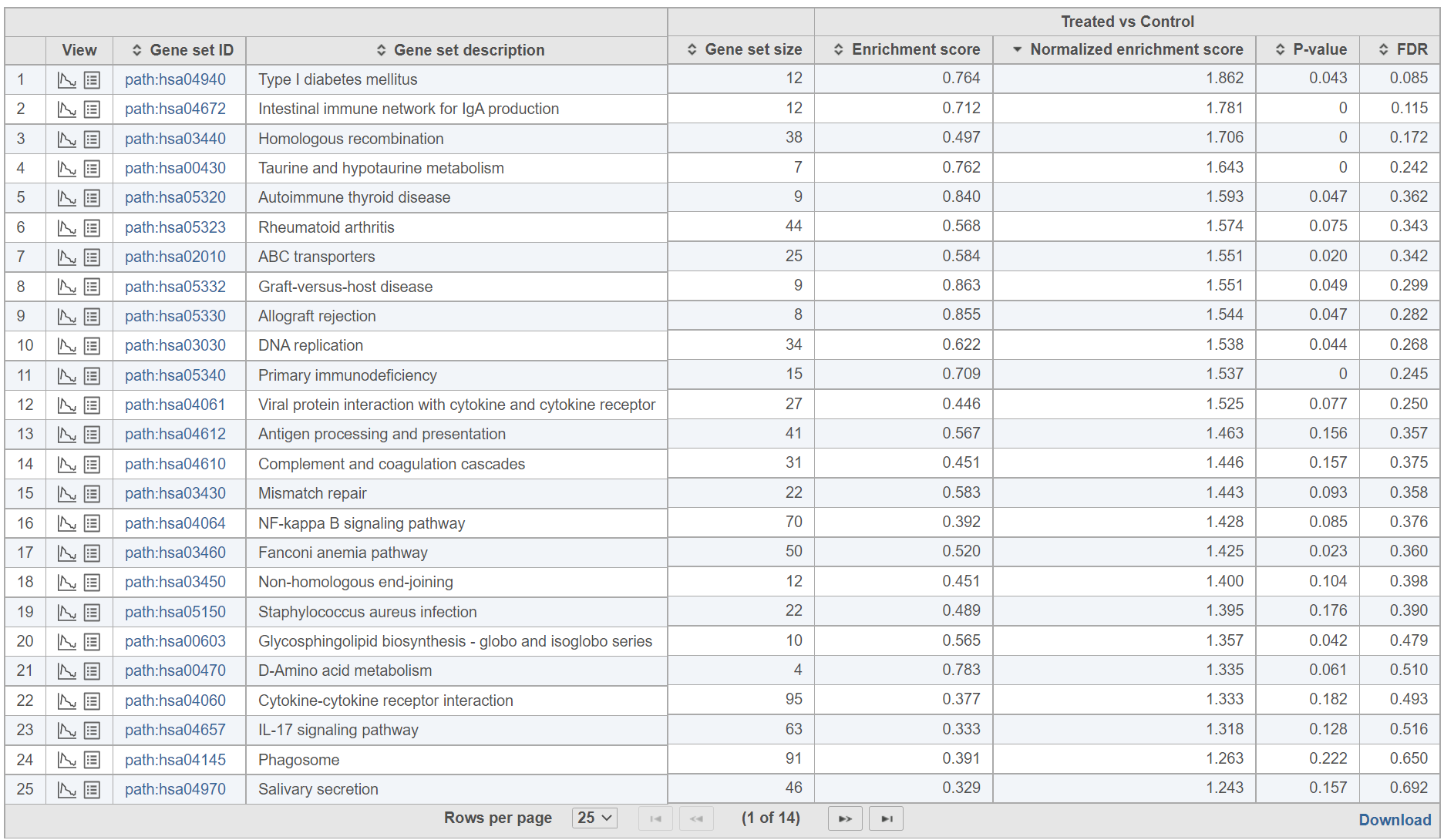
The comparison (i.e. Denominator vs. Numerator) is given at the top of the GSEA table. To download the table to your local computer as a text file, use the Download link in the bottom right. Each row of the table corresponds to one gene set and the gene sets are ranked by the P-value, ascending (lowest values at the top). The icon (![]() ) in the column headers are used for sorting. The columns of the table are as follows.
) in the column headers are used for sorting. The columns of the table are as follows.
...
| Numbered figure captions | ||||
|---|---|---|---|---|
| ||||
|
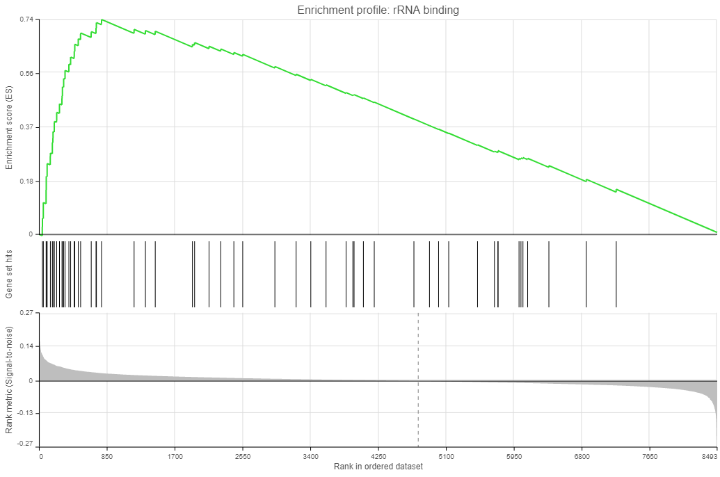
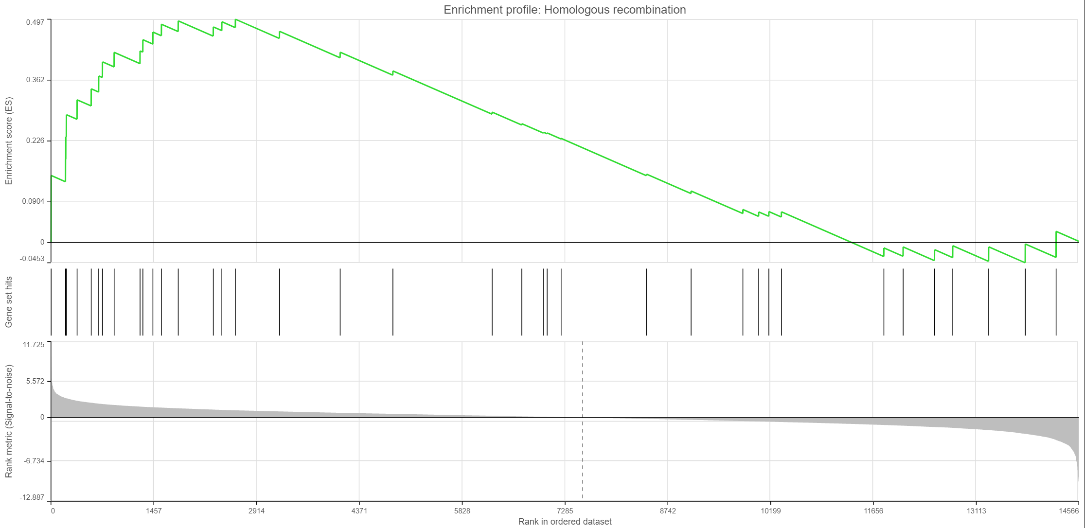
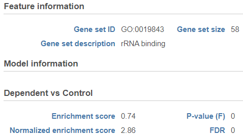
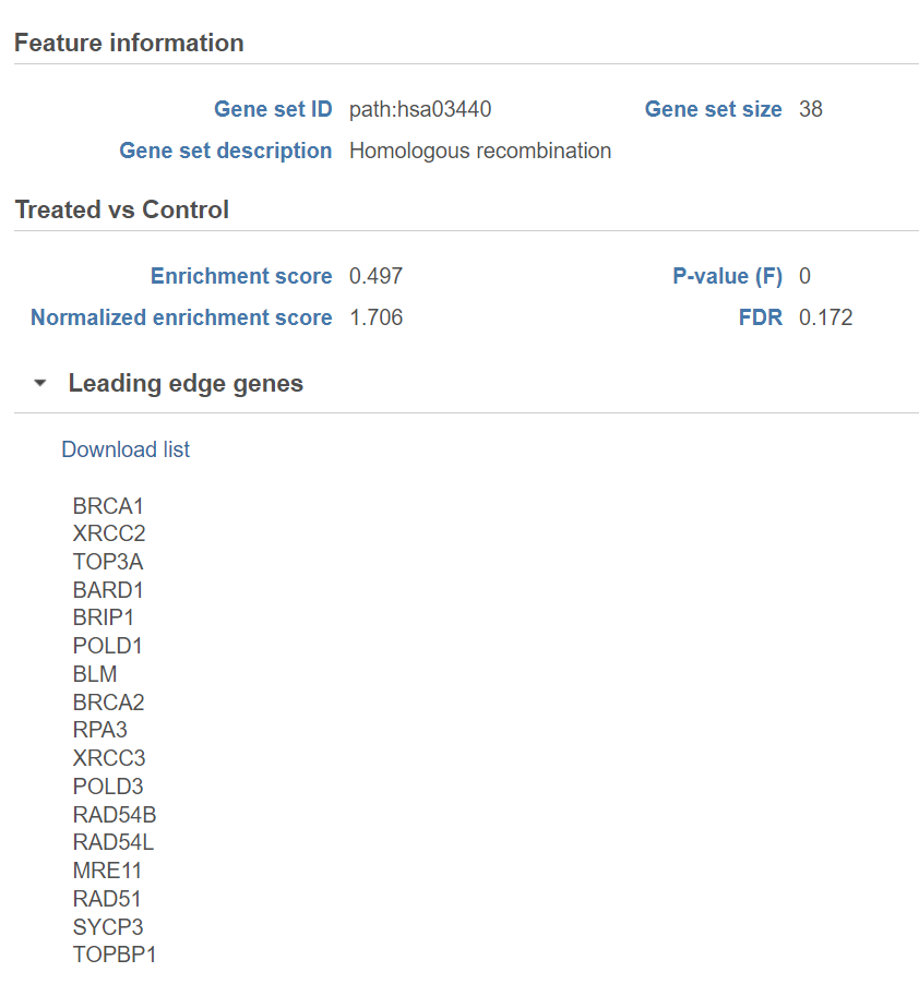
Click on the View extra details plot (![]() ) to open a gene set-specific report page (Figure 12).
) to open a gene set-specific report page (Figure 12).
Leading edge genes: it is a subset of genes that contribute most to the ES. For a positive ES, the leading edge subset is the set of members that appear in the ranked list prior to the peak score. For a negative ES, it is the set of genes that appear subsequent to the peak score.
| Numbered figure captions | ||||
|---|---|---|---|---|
| ||||
|
References
- Subramanian A, Tamayo P, Mootha VK, et al. Gene set enrichment analysis: a knowledge-based approach for interpreting genome-wide expression profiles. Proc Natl Acad Sci U S A. 2005;102(43):15545-15550. doi:10.1073/pnas.0506580102
- Mootha VK, Lindgren CM, Eriksson KF, et al. PGC-1alpha-responsive genes involved in oxidative phosphorylation are coordinately downregulated in human diabetes. Nat Genet. 2003;34(3):267-273. doi:10.1038/ng1180
Overview
Content Tools