Page History
...
Differential expression analysis can be used to compare cell types. Here, we will compare glioma and oligodendrocyte cells to identify genes differentially regulated in glioma cells from the Oligodendroglioma oligodendroglioma subtype. Glioma cells in Oligodendroglioma oligodendroglioma are thought to originate from oligodendrocytes; , thus directly comparing the two cell types will identify genes that distinguish them.
Filter
...
cells
To analyze only the Oligodendroglioma oligodendroglioma subtype, we can filter the samples.
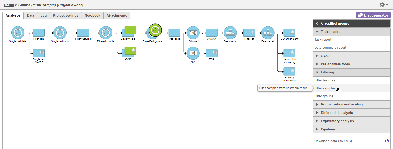
- Click the green Classified groups Filtered counts data node
- Click Expand Filtering in the task menu
- Click Filter samples cells (Figure 1)
| Numbered figure captions | ||||
|---|---|---|---|---|
| ||||
|
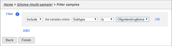
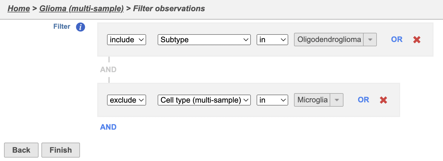
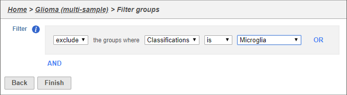
The filter lets us include or exclude samples based on sample ID and attribute.
- Set the filter to Include samples where Subtype is Oligodendroglioma
- Click AND
- Set the second filter to exclude Cell type (multi-sample) is Microglia
- Click Finish to apply the filter (Figure 2)
...
...
| Numbered figure captions | ||
|---|---|---|
|
...
|
...
|
...
- Set the filter to Include samples where Subtype is Oligodendroglioma
- Click Finish to apply the filter
...
|
A Filtered counts data node will be created with only cells that are from Oligodendroglioma oligodendroglioma samples (Figure 3).
| Numbered figure captions | |
|---|---|
|
...
| Numbered figure captions | ||||
|---|---|---|---|---|
| ||||
|
A Filtered Counts data node will be created with only glioma and oligodendrocyte cells from the Oligodendroglioma samples. The Filtered groups task must complete before we can proceed to identifying differentially expressed genes.
|
...
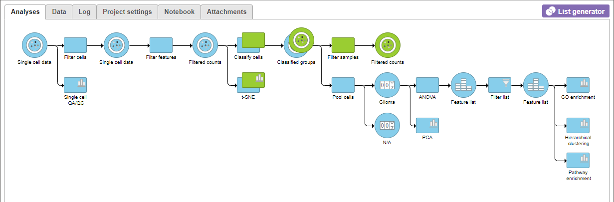
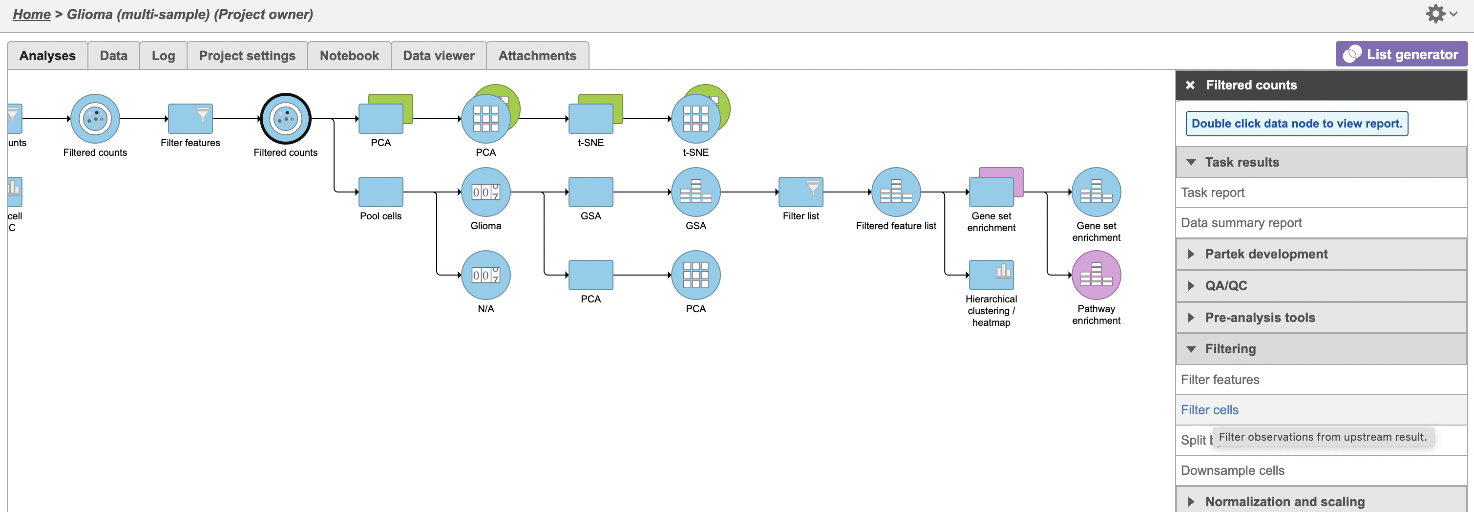
Filter groups
Because we are only interested in analyzing glioma and oligodendrocyte cells, we will filter out microglia cells using the groups filer.
- Click the green Filtered counts data node
- Click Filtering in the task menu
- Click Filter groups
This filter lets us include or exclude cells based on classifications or other cell-level attributes.
...
|
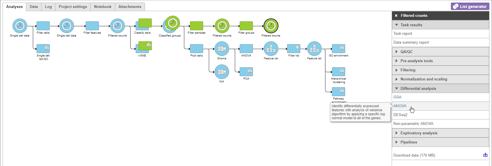
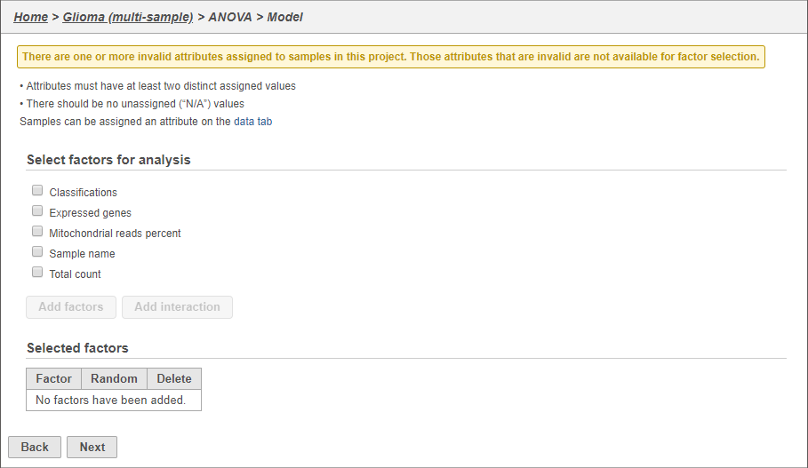
Identify differentially expressed genes
- Click the second green Filtered new Filtered counts data node
- Click Click Statistics > Differential analysis in the task menu
- Click ANOVA (Figure 5)
| Numbered figure captions | ||||
|---|---|---|---|---|
| ||||
|
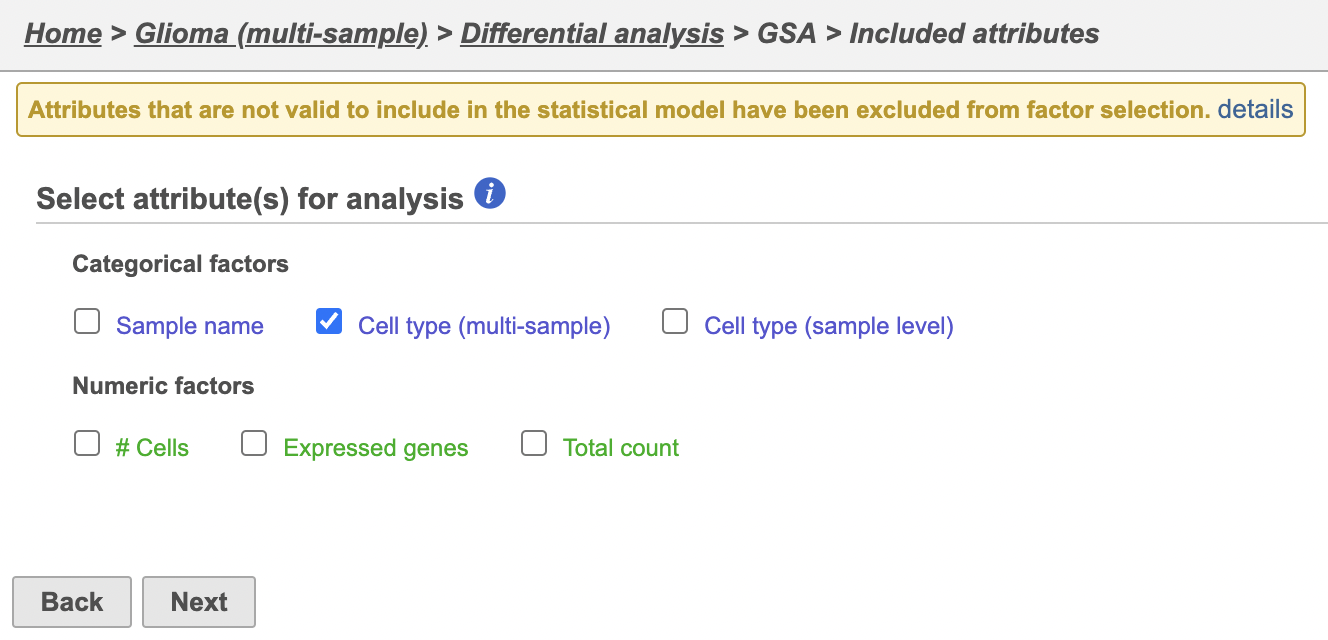
- GSA
The configuration options (Figure 64) include includes sample and cell-level attributes. Here, we want to compare different cell types so we will include Classification Cell type (multi-sample).
- Click Cell type (multi-sample)
- Click Next
| Numbered figure captions | |
|---|---|
|
...
|
...
|
...
- Click Classification
- Click Add factors
- Click Next
...
|
Next, we will set up a comparison between gliioma glioma and oligodendrocytesoligodendrocyte cells.
- Click Glioma Click the arrow to move it to the top-right in the top panel
- Click OligodendrocytesClick the arrow to move it to the top-right bottom-right Oligodendrocytes in the bottom panel
- Click Add comparison (Figure 85)
This will set up fold calculations with glioma as the numerator and oligodendrocytes as the denominator.
| Numbered figure captions | ||||
|---|---|---|---|---|
|
...
|
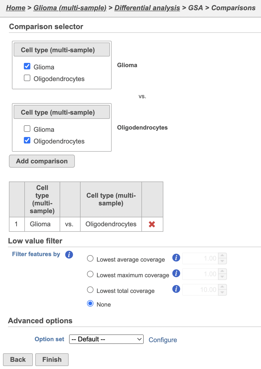
- Click None in the Read count normalization sectionClick Finish to run the ANOVAGSA
A green Feature list node GSA data node will be generated containing the results of the ANOVAGSA.
- Double-click the green Feature list node the green GSA data node to open the ANOVA GSA report
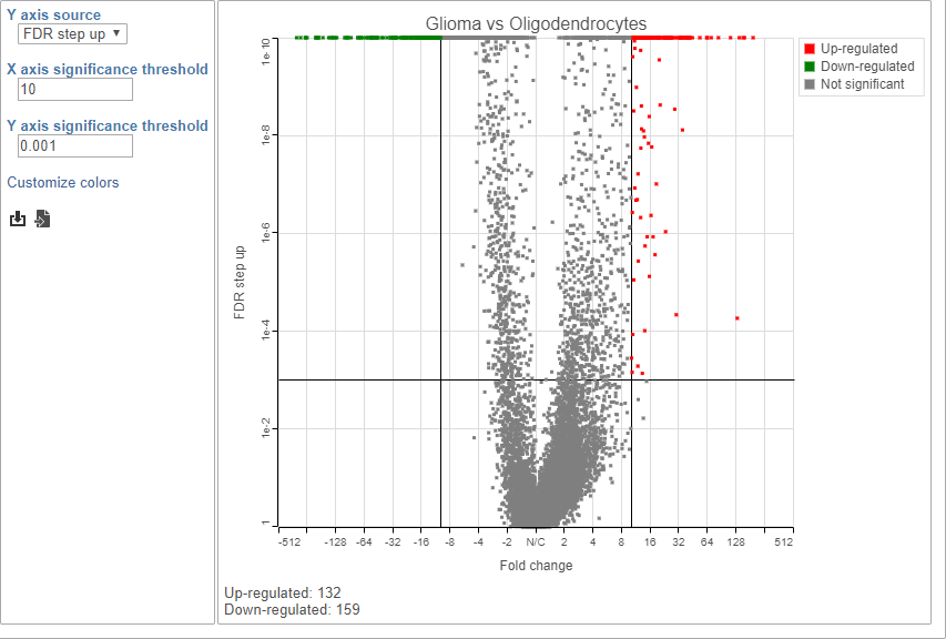
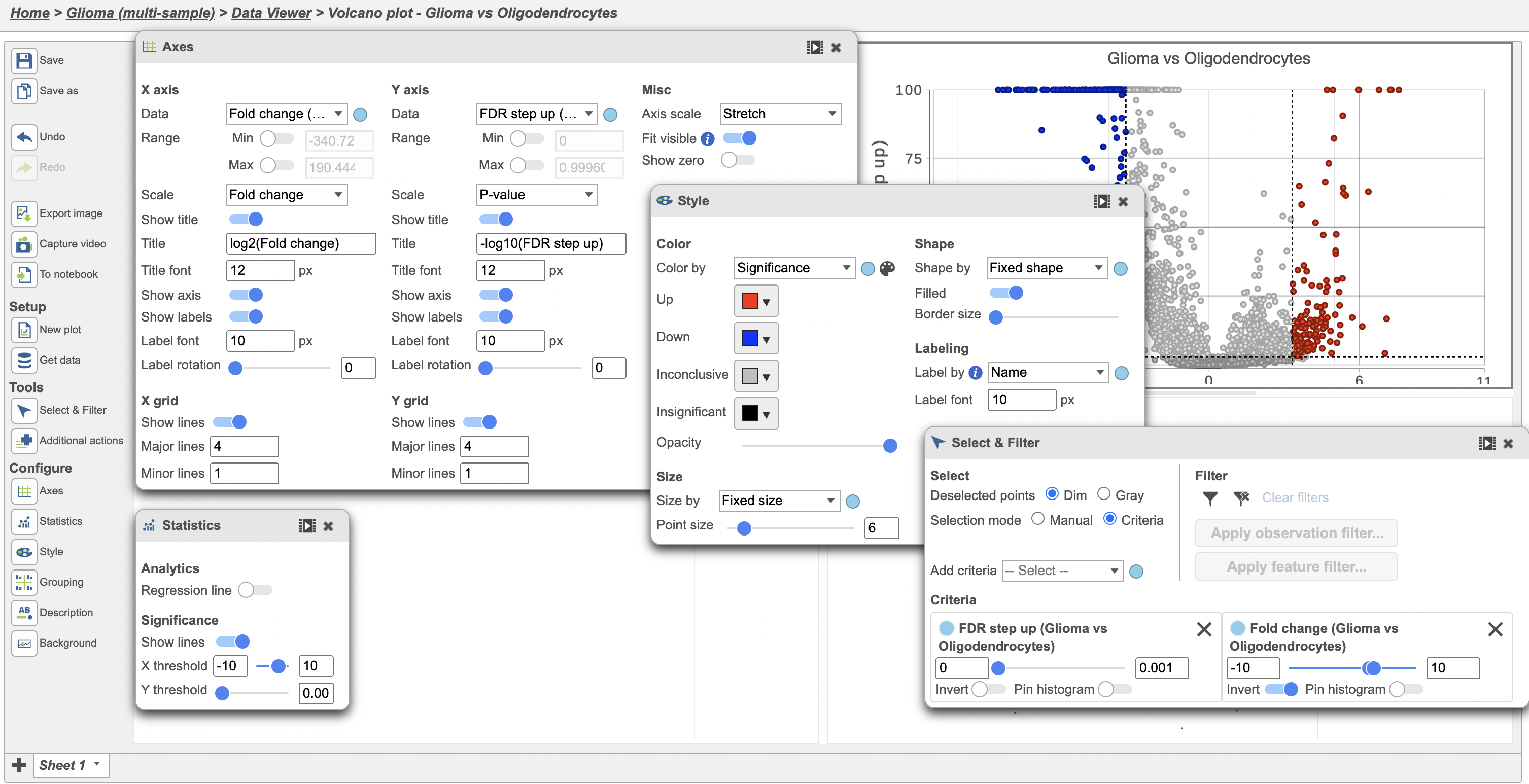
Because of the large number of cells and large differences between cell types, the p-values and FDR step up values are very low for highly significant genes. We can use the volcano plot to preview the effect of applying different significance thresholds.
- Click
 to view the Volcano plot
 - Choose FDR step up from the Y axis source drop-down menu
- Set the X axis significance thresold to 10
- Set the Y axis significance thresold to 0.001
This gives 132 up-regulated and 159 down-regulated genes (Figure 9).
- Open the Style icon on the left, change Size point size to 6
- Open the Axes icon on the left and change the Y-axis to FDR step up (Glioma vs Oligodendrocytes)
- Open the Statistics icon and change the Significance of X threshold to -10 and 10 and the Y threshold to 0.001
- Open the Select & Filter icon, set the Fold change thresholds to -10 and 10
- In Select & Filter, click
 to remove the P-value (Glioma vs Oligodendrocytes) selection rule. From the drop-down list, add FDR step up (Glioma vs Oligodendrocytes) as a selection rule and set the maximum to 0.001
Note these changes in the icon settings and volcano plot below (Figure 6).
| Numbered figure captions | ||||
|---|---|---|---|---|
| ||||
|
We can now recreate these conditions in the ANOVA GSA report filter.
- Click ANOVA report at the top of the screen GSA report tab in your web browser to return to the ANOVA GSA report
- Click FDR step up
- Set the FDR step up filter to Less than or equal to 0.001
- Press Enter
- Click Fold change
- Set the Fold change filter to From -10 to 10
- Press Enter
The filter should include 291 genes.
- Click
 to apply the filter and generate a filtered Filtered Feature list nodelist node
Exploring differentially expressed genes
To visualize the results, we can generate a hierarchical clustering heat mapheatmap.
- Click the second green Feature list Filtered feature list produced by the Differential analysis filter task
- Click Exploratory analysis in the task menu
- Click Hiearchical clustering Click Hierarchical clustering/heatmap
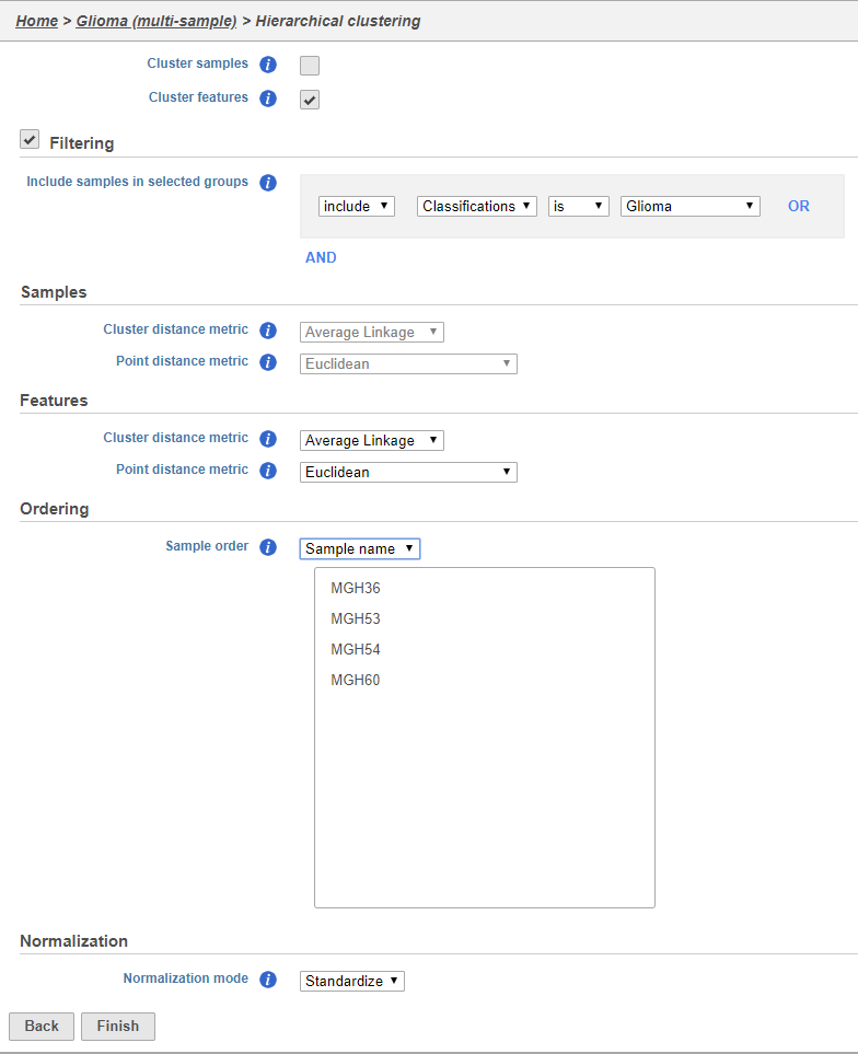
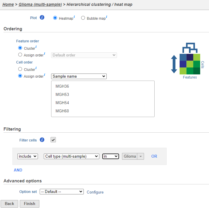
Using the hierarchical clustering options we can choose to include only cells from certain samples. We can also choose the order of cells on the heat map heatmap instead of clustering. Here, we will include only glioma cells and order the samples by sample ID name (Figure 107).
- Uncheck Cluster samples
- Click Filtering and Make sure Cluster is unchecked for Cell order
- Click Filter cells under Filtering and set the filter to include Classifications Cell type (multi-sample) is Glioma
- Choose Sample name from the Sample order Choose Sample name from the Cell order drop-down menu in the Ordering Assign order section
- Click Finish
| Numbered figure captions | ||||
|---|---|---|---|---|
| ||||
|
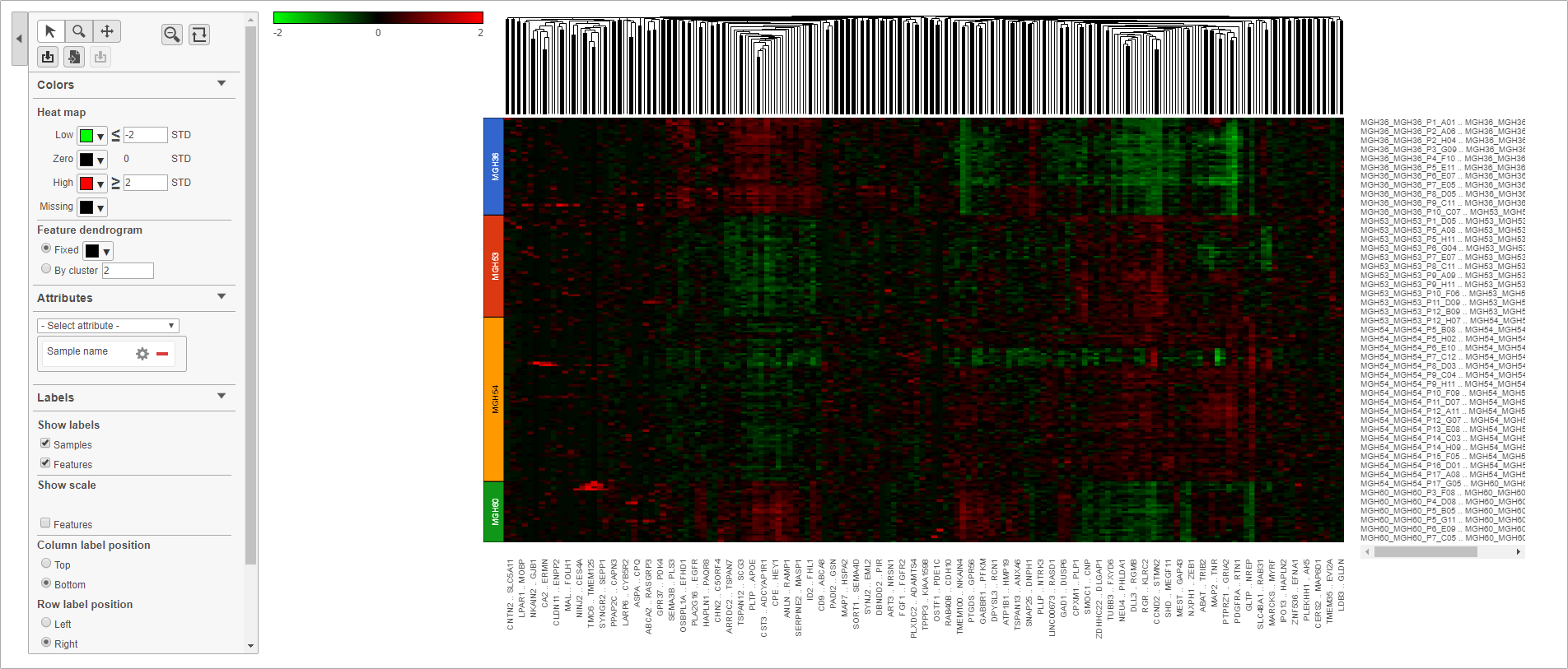
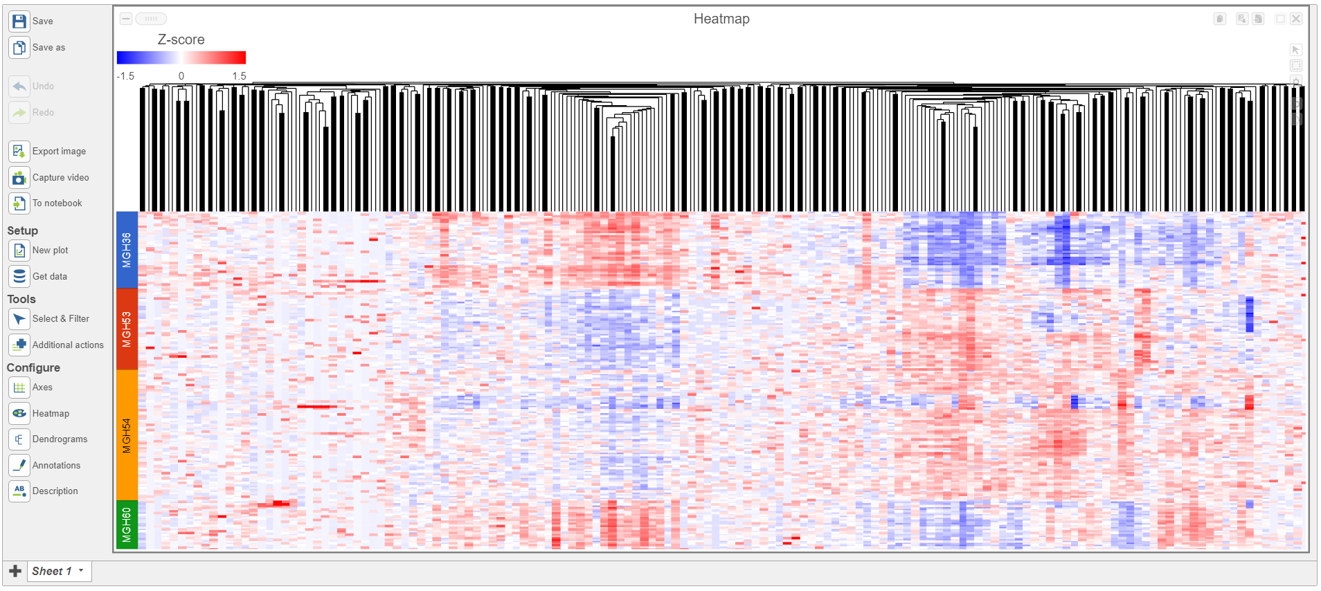
- Double click the green Hierarchical clustering node to open the heat mapheatmap
The heat map will appear black heatmap differences may be hard to distinguish at first; the range from red to green blue with a black white midpoint is set very wide because of a few outlier cells. We can adjust the range to make more subtle differences visible. We can also adjust the color.
- Set Low Set the Range toggle Min to -2
- Set High to 2
...
- 1.5
- Set the Range toggle Max to 1.5
The heatmap now shows clear patterns of red and greenblue.
- Click Axis titles and deselect the Row labels and Column labels of the panel to hide sample and feature names, respectively.
- Select Sample name from the Attributes Annotations drop-down menu
Cells are now labeled with their sample name. Interestingly, samples show characteristic patterns of expression for these genes (Figure 118).
| Numbered figure captions | ||||
|---|---|---|---|---|
| ||||
|
- Click Glioma (multi-sample) to return to the pipeline view Analyses tab.
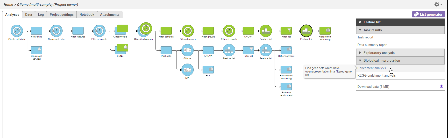
We can use GO gene set enrichment to futher further characterize the differences between glioma and oligodendrocyte cells.
- Click the second green Feature Filtered feature list node
- Click Biological interpretation in the task menu
- Click Enrichment anlaysis (Figure 12)
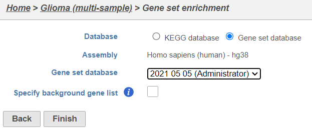
- Click Gene set enrichment
- Change Database to Gene set database and click Finish to continue with the most recent gene set (Figure 9)
| Numbered figure captions | ||||
|---|---|---|---|---|
| ||||
|
- Choose Homo sapiens (human) - hg38 from the Assembly drop-down menu
- Select Finish to continue with the most recentgene set
...
|
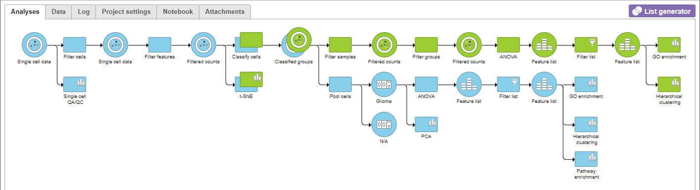
A Gene set enrichment node will be added to the pipeline view (Figure 13) .
| Numbered figure captions | ||||
|---|---|---|---|---|
| ||||
|
- Double-click the green GO the Gene set enrichment task node to open the task report
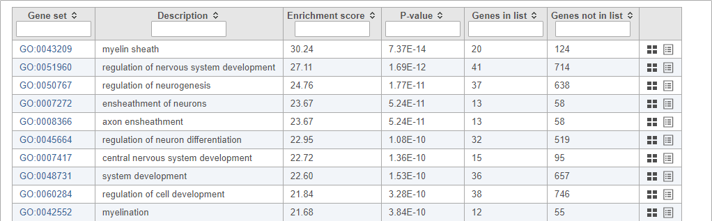
Top GO terms in the enrichment report include "myelin sheath", "ensheathment of neurons" , and "axon ensheathment" (Figure 1410), which corresponds well with the role of oligodendrocytes in creating the myelin sheath that supports and protect axons in the central nervous system.
| Numbered figure captions | ||||
|---|---|---|---|---|
| ||||
|
...
| Additional assistance |
|---|
| Rate Macro | ||
|---|---|---|
|
...
Overview
Content Tools