Page History
Although the 450K and MethylationEPIC arrays were initially designed to analyze DNA methylation, they are essentially a dense SNP array and can thus be used for copy number analysis (Feber et al. 2014). The probe intensity data is easily parsed from the idat files by using the Additional Probe Data Spreadsheet Selection dialog (Figure 1) when importing the raw data. Examining the raw intensity data can also be useful for QA/QC purposes.
Follow the steps for importing Illumina methylation data until detailed in Import and normalize methylation data until you reach the Import Illumina iDAT Data dialog with Manifest File and Output File panels (Figure 1).
...
| Numbered figure captions | ||||
|---|---|---|---|---|
| ||||
|
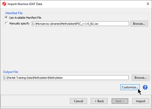
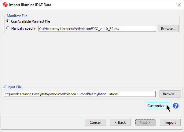
- Select Customize... to open the Advanced Import Options dialog
- Choose No normalization in the Normalization section of the Algorithm tab
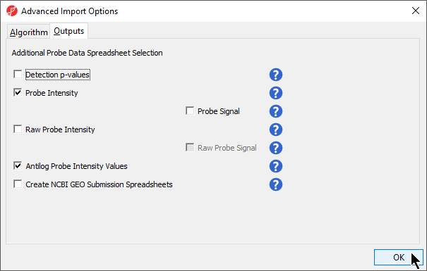
- Select the Outputs tab (Figure 2)
| Numbered figure captions | ||||
|---|---|---|---|---|
| ||||
|
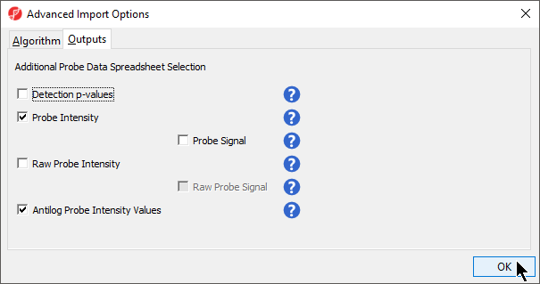
Information about the different output options can be found by selecting the adjacent (![]() ) icon.
) icon.
Detection p-values. This is the confidence score that the signal of a probe was significantly higher than the background defined by negative control probes. Selecting this checkbox produces a spreadsheet ending with '_detectionp' in addition to the spreadsheet containing beta values. Each row of the _detectionp spreadsheet will be a different sample and the sample names will end in '_detectionp'. This spreadsheet can be used to filter out probes that do not show signal above background.
Probe Intensity. This is the sum of the methlyated and unmethylated intensities per probe. Selecting this checkbox produces a spreadsheet ending with ‘_probe’ in addition to the spreadsheet containing beta values. Each row of the _probe spreadsheet will be a different sample and the file names will also end in ‘_probe.’ The probe intensity values will be log2 transformed by default (note that the beta values are not log2 transformed).
Probe Signal. This option will become available if Probe Intensity is selected. Selecting this checkbox produces a spreadsheet ending with ‘_probe.’ The methylated and unmethylated intensities are shown on separate rows for each sample, in addition to the summed values. The sample names will end in ‘_meth’ or ‘_unmeth’ for methylated and unmethylated values, respectively. The probe intensity values will be log2 transformed by default.
Raw Probe Intensity. This is the sum of the raw red and green signal intensities per probe. Selecting this checkbox produces a spreadsheet ending with ‘_raw’ in addition to the spreadsheet containing beta values. Each row of the spreadsheet will be a different sample and the file names will also end in ‘_raw.’ The raw probe intensity values will be log2 transformed by default.
Raw Probe Signal. This option will become available if Raw Probe Intensity is selected. Selecting this checkbox produces a spreadsheet ending with ‘_raw.’ The red and green intensities will be shown on separate rows for each sample, in addition to the summed values. The sample names will end in ‘_red’ or ‘_green’ for red and green values, respectively. The raw probe intensity values will be log2 transformed by default.
Antilog Probe Intensity Values. Selecting this checkbox will show the probe intensity data without log2 transformation.
Create NCBI GEO Submission Spreadsheets. Generates matrix processed and matrix signal intensities spreadsheets for GEO submission.
How you proceed depends on your study design. Here is an example series of steps to prepare the tutorial data set for copy number analysis:
- Select Probe Intensity and Antilog Probe Intensity Values (Figure 2)
- Select OK to close the Advanced Import Options dialog
- Select Import to import the data and perform the selected normalization method
- Select the (_probe) spreadsheet from the spreadsheet tree
- Delete any samples with _detectionp names
- Create sample attributes , and assign samples to the groups , and filter as described in Annotate and Filter Samplessamples
- Select Transform from the main toolbar
- Select Normalize to baseline
...
This spreadsheet contains copy number values per probe in log2 space (i.e. diploid = 0). This Prior to performing copy number analysis, you can normalize for local GC abundance.
- Select Transform
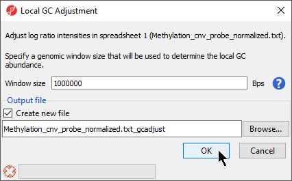
- Select Adjust Based on Local GC Content...
- Click OK to run Local GC Adjustment (Figure 4)
| Numbered figure captions | ||||
|---|---|---|---|---|
| ||||
|
References
...
Feber A, Guilhamon P, Lechner M, et al. Using high-density DNA methylation arrays to profile copy number alterations. Genome Biology. 2014;15(2):R30. doi:10.1186/gb-2014-15-2-r30.
...
Overview
Content Tools