Page History
...
| Table of Contents | ||||||
|---|---|---|---|---|---|---|
|
ANOVA dialog
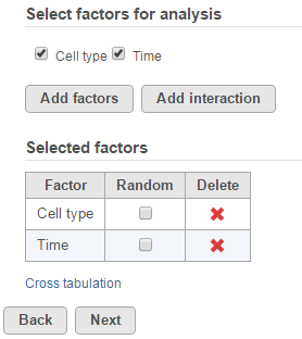
To setup ANOVA model or the alternative Welch's ANOVA (which is used on normally distributed data that violates the assumption of homogeneity of variance), select factors from sample attribute. The factors can be categorical or numeric attribute. Click on a check button to select and click Add factors button to add it to the model (Figure 1).
LIMMA-trend and LIMMA-voom setup dialogs are identical to ANOVA's setup.
Note: LIMMA-voom method can only be invoked on the following normalization output data node, those methods can produce library sizes:
TMM, CPM, Upper Quartile, Median ratio, Postcounts
| Numbered figure captions | ||||
|---|---|---|---|---|
| ||||
|
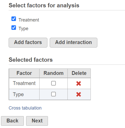
When more than one factor is selected, click Add interaction button will be enabled to allow you to specify interactionto add interaction term of the selected factors.
Once a factor is added to the model (Figure 14), you can specify whether the factor is a random effect (check Random check box) or not.
Most factors in an analysis of variance are fixed factors, i.e. the levels of that factor represent all the levels of interest. Examples of fixed factors include gender, racetreatment, straingenotype, etc. However, in experiments that are more complex, a factor can be a random effect, meaning the levels of the factor only represent a random sample of all of the levels of interest. Examples of random effects include subject and batch.Consider Consider the example where one factor is type (with levels normal and diseased), and another factor is subject (the subjects selected for the experiment). In this example,
“type” “Treatment” is a fixed factor since the levels normal treated and diseased control represent all conditions of interest. “Subject”, on the other hand, is a random effect since the subjects are only a random sample of all the levels of that factor. When model has both fixed and random effect, it is called a mixed model.
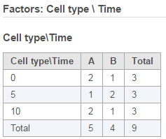
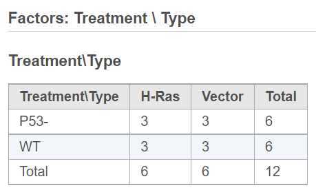
When more than one factor is added to the model, click on the Cross tabulation link at the bottom to view the relationship between the factors in a different browser tab (Figure 2).
| Numbered figure captions | ||||
|---|---|---|---|---|
| ||||
|
Once the model is set, click on Next button to setup comparisons (contrasts) (Figure 3).
| Numbered figure captions | ||||
|---|---|---|---|---|
| ||||
|
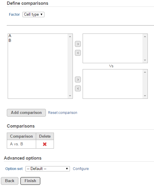
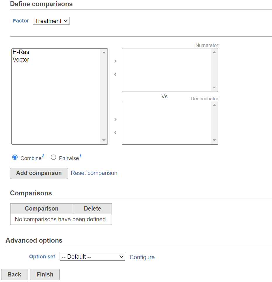
Start by choosing a factor or interaction from the Factor drop-down list. The subgroups of the factor or interaction will be displayed in the left panel; click to select one or more more level(s) or subgroup name(s) and move them to one of the panels boxes on the right. The ratio/fold change calculation on the comparison will use the group in the top panel box as numerator, and the group in the bottom panel box as the denominator. Click When multiple levels (groups) are in either numerator or denominator box(es), in Combine mode, click on Add comparison button to add one comparison to the comparisons table. Note that multiple comparisons can be added to combine all numerator levels and combine all denominator levels in a single comparison in the Comparison table below; in Pairwise, click on Add comparison button will split all numerator levels and denominator levels into a factorial set of comparisons – in other words, it will add every numerator level paired with every denominator level comparisons to the Comparison table . Multiple comparisons from different factors can be added from the specified model.
ANOVA advanced options
Click on the Configure to customize Advanced options (Figure 4)
| Numbered figure captions | ||||
|---|---|---|---|---|
| ||||
|
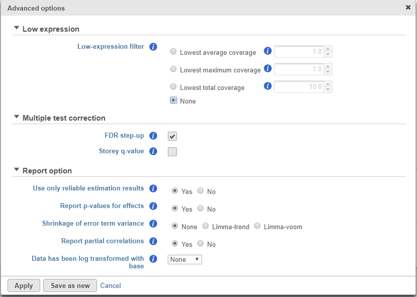
Low-expression feature and Multiple test correction sections are the same as the matching GSA advanced option, see above GSA advanced options.
...
Use only reliable estimation results: There are situations when a model estimation procedure does not fail outright, but still encounters some difficulties. In this case, it can even generate p-value and fold change on the comparisons, but they are not reliable, i.e. they can be misleading. Therefore, the default of Use only reliable estimation results is set Yes.
Report p-value for effects: If set to No, only the p-value of comparison will be displayed on the report, the p-value of the factors and interaction terms are not shown in the report table. When you choose Yes in addition to the comparison’s p-value, type III p-values are displayed for all the non-random terms in the model.
Shrinkage to error term variance: by default, None is select, which is lognormal model. Limma-trend and Limma-voom options are lognormal with shrinkage. (Limma-trend is the same as the GSA default option–lognormal with shrinkage). Shrinkage options are recommended for small sample size design, no random effects can be included when performing shrinkage. If there are numeric factors in the model, the partial correlations cannot be reported on the numeric factors when shrinkage is performed. Limma-trend works well if the ratio of the largest library size to the smallest is not more than 3 fold, it is simple and robust for any type of data. Limma-voom is recommended for sequencing data when library sizes vary substantially, but it can only be invoked on data node normalized using TMM, CPM, or Upper quartile methods while Limma-trend can be applied to normalized data using any method.
Report partial correlations: If the model has a numeric factor(s), when choosing Yes, partial correlation coefficient(s) of the numeric factor(s) will be displayed in the result table. When choosing No, partial correlation coefficients are not shown.
Data has been log transformed with base: showing the current scale of the input data on this task.
ANOVA report
Since there is only one model for all features, so there is no pie charts design models and response distribution information. The Gene list table format is the same as the GSA report.
References
- Benjamini, Y., Hochberg, Y. (1995). Controlling the false discovery rate: a practical and powerful approach to multiple testing, JRSS, B, 57, 289-300.
- Storey JD. (2003) The positive false discovery rate: A Bayesian interpretation and the q-value. Annals of Statistics, 31: 2013-2035.
- Auer, 2011, A two-stage Poisson model for testing RNA-Seq
- Burnham, Anderson, 2010, Model selection and multimodel inference
- Law C, Voom: precision weights unlock linear model analysis tools for RNA-seq read counts. Genome Biology, 2014 15:R29.
- http://cole-trapnell-lab.github.io/cufflinks/cuffdiff/index.html#cuffdiff-output-files
- Anders S, Huber W: Differential expression analysis for sequence count data. Genome Biology, 2010
...
| Additional assistance |
|---|
| Rate Macro | ||
|---|---|---|
|
...
Overview
Content Tools