Page History
With the Partek ® Flow ® Microarray Toolkit, you can import and analyze microarray data with the same ease as any sequencing analysis pipeline. This document covers the following parts.
...
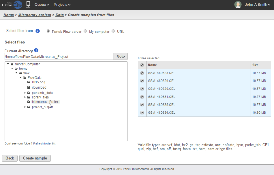
The most efficient way of importing array data would be to import them directly from your Partek Flow server. When you select this option, navigate to the folder containing your data files. Valid file types will be selectable for upload. Click on the files you would like to import into the project and select the Create sample button (Figure 1).
| Numbered figure captions | ||||
|---|---|---|---|---|
| ||||
|
...
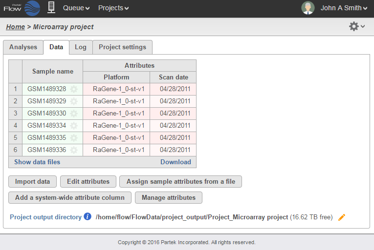
Once the samples have been uploaded, the Data tab will list each sample along with the Platform associated with each sample. If Affymetrix .CEL files were uploaded, it will also include the date that the array was scanned (Figure 2). This information may be helpful in assessing possible batch effects.
| Numbered figure captions | ||||
|---|---|---|---|---|
| ||||
|
...
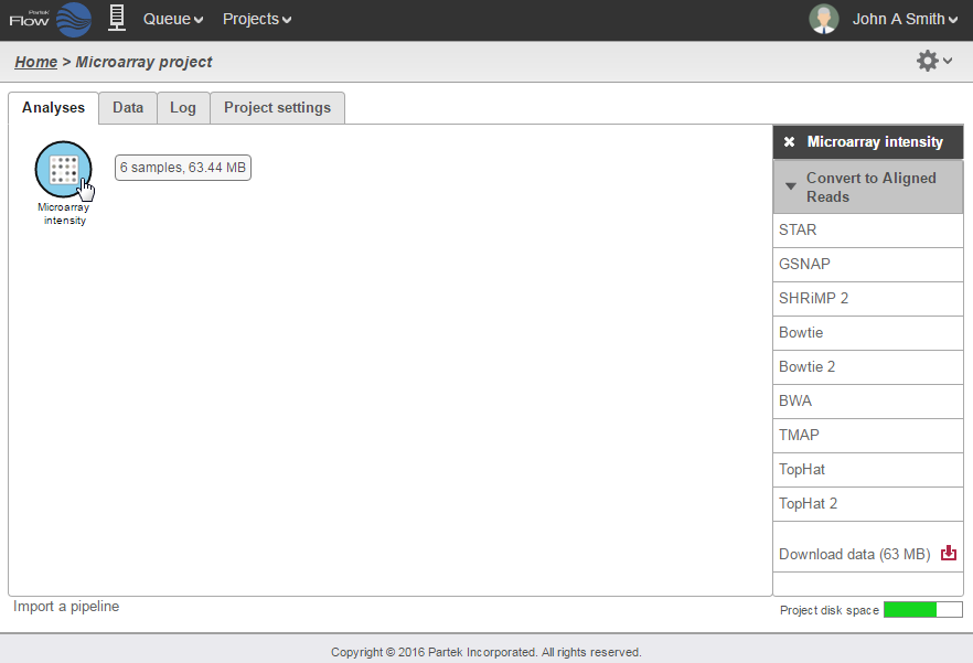
Once the microarray data has been uploaded, the Microarray intensity data node will appear in the Analyses tab. To convert this data to aligned reads, select the Microarray intensity data node and select the aligner you would like to use for conversion (Figure 3).
| Numbered figure captions | ||||
|---|---|---|---|---|
| ||||
|
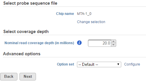
Selecting an aligner will bring up the Microarray Conversion options page (Figure 4). Under the Select probe sequence file section, make sure that the correct Chip name is specified. For non-custom arrays, these should be set automatically to the platform detected upon importing the array.
| Numbered figure captions | ||||
|---|---|---|---|---|
| ||||
|
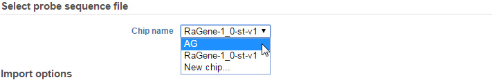
If for some reason you wish to override that selection, then click the Change selection link and select the chip name in the drop-down menu or select New chip… if you would like to upload a different chip annotation (Figure 5).
| Numbered figure captions | ||||
|---|---|---|---|---|
| ||||
|
...
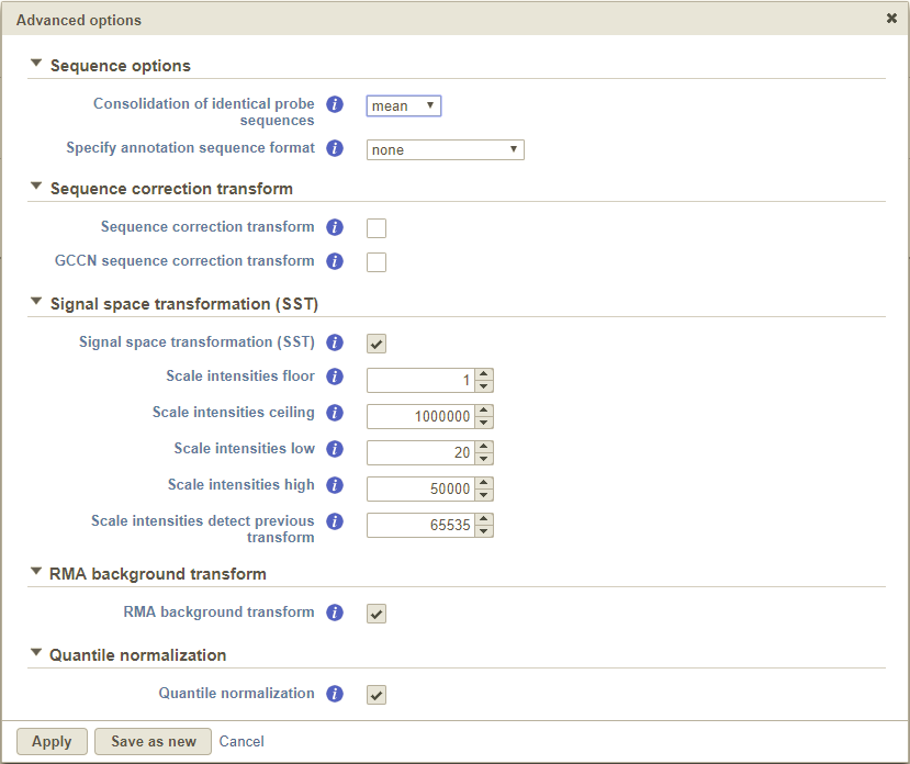
Clicking the Configure link under the Advanced options section to view the advanced options that can be modified. These are generally transformations applied to microarray data (Figure 6). Note that both interrogating and control (if present) probes are used during fitting and adjustment.
| Numbered figure captions | ||||
|---|---|---|---|---|
| ||||
|
...
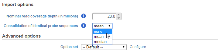
By default, this is set to take the mean of the intensities the probes and utilizes that to calculate the read count for the probe sequence. Clicking on the drop-down menu allows you to either turn off this feature (none) or use the median instead (Figure 6).
| Numbered figure captions | ||||
|---|---|---|---|---|
| ||||
|
...
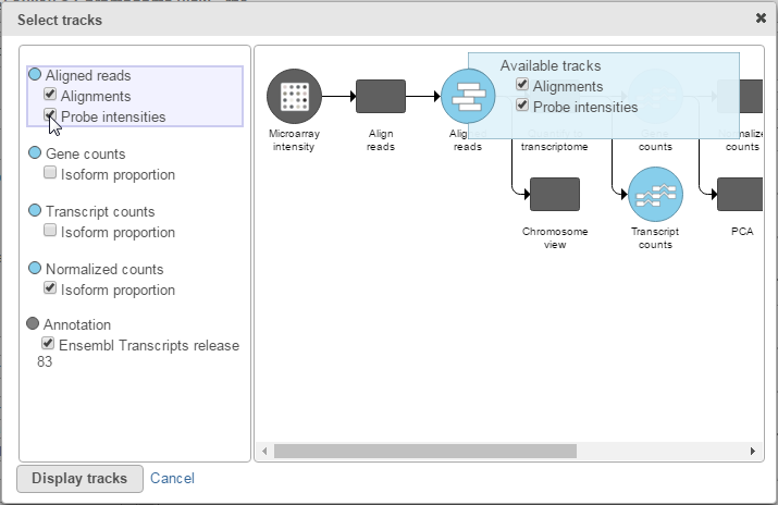
To visualize microarray probes in Partek Flow's Chromosome viewer, click the Select tracks button at the top left corner of the viewer. Select the Probe intensities check box to display microarray probes (Figure 8).
| Numbered figure captions | ||||
|---|---|---|---|---|
| ||||
|
This will display microarray probes aligned to the reference genome (Figure 9). By default, the probes are colored by their intensities with darker shades signifying higher probe intensities.
| Numbered figure captions | ||||
|---|---|---|---|---|
| ||||
...
- Affymetrix Whitepaper on Microarray normalization using Signal Space Transformation with probe Guanine Cytosine Count Correction. Accessed February 17, 2016
- Irrizarry RA, Hobbs B, Collin F et al. Exploration, normalization, and summaries of high density oligonucleotide array probe level data. Biostat. 2003; 4:249-264.
...
...
| Additional assistance |
|---|
| Rate Macro | ||
|---|---|---|
|
...
Overview
Content Tools