Page History
...
| Numbered figure captions | ||||
|---|---|---|---|---|
| ||||
...
Multiple comparisons can be computed in one GSA run,; Figure 5 is showing shows the above three comparisons are added in the computation.
...
The more comparisons on different terms are added, the fewer models will be included in the computation. if If the following comparisons are added in one GSA run:
- A vs B (Cell type)
- 5 vs 0 (Time)
...
| Numbered figure captions | ||||
|---|---|---|---|---|
| ||||
...
| Numbered figure captions | ||||
|---|---|---|---|---|
| ||||
...
This section configures how to select the best model for a feature. There are two options for Model selection criterion: AICc (Akaike Information Criterion corrected) and AIC (Akaike Information Criterion). AICc is recommended for small sample size, while AIC is recommended for medium and large sample size What about large samples?(3). Note that when sample size grows from small to medium, AICc converges to AIC. Taking the AICc/AIC value into account, GSA considers the model with the lowest information criterion as the best choice.
In the results, the best model's Akaike weight is also generated. The model's weight is interpreted as the probability that the model would be picked as the best if the study were reproduced. The range of Akaike weight is between 0 to 1, where 1 means the best model is very superior to the other candidates from the model pool; if the best model's Akaike weight is close to 0.5 on the other hand, it means the best model is likely to be replaced by other candidates if the study were reproduced. One still uses the best shot model, however, the accuracy of the best shot is fairly low.
...
- Normal
- Lognormal (the same as ANOVA task)
- Lognormal with shrinkage (the same as limma-trend method 54)
- Negative binomial
- Poisson
We recommend to use lognormal with shrinkage distribution (the default), and an experienced user may want to click on Custom to configure the model type and p-value type (Figure 8).
...
Partek Flow keeps tracking the log status of the data, and no matter whether GSA is performed on logged data or not, the fold change calculation is always in linear scale
...
If lognormal with shrinkage method was selected for GSA, a shrinkage plot is generated in the report (Figure 13). X-axis shows the log2 value of average coverage. The plot helps to determine the threshold of low expression features. X-axis shows the log2 value of average coverage. If there is an increase before a monotone decrease trend on the left side of the plot, you need to set a higher threshold on the low expression filter, detailed . Detailed information on how to set the threshold can be found from in the GSA white paper.
| Numbered figure captions | ||||
|---|---|---|---|---|
| ||||
...
| Numbered figure captions | ||||
|---|---|---|---|---|
| ||||
When more than one factors are factor is selected, Add interaction button will be enabled to allow you to specify interaction.
Once the a factor is added to the model (Figure 14), you can specify whether the factor is random effect or not. Not checking the Random check button will be treated as fixed effect.a random effect (check Random check box) or not.
Most factors in an analysis of variance are fixed factors, i.e. the levels of that factor represent all the levels of interest. Examples of fixed factors include gender, race, strain, etc. However, in experiments that are more sophisticated complex, a factor can be a random effect, meaning the levels of the factor only represent a random sample of all of the levels of interest. Examples of random effects include subject and batch.
Consider the example where one factor is type (with levels normal , and diseased), and another factor is subject (the subjects selected for the experiment). In this example, type
“type” is a fixed factor since the levels normal and diseased represent all conditions of interest. Subject on “Subject”, on the other hand, is a random effect since the subjects are only a random sample of all the levels of that factor. When a model model has both a fixed and random effect, it is called a mixed - model.
When more than one factor is added to the model, click on the Cross tabulation link at the bottom to view the relationship between the factors (Figure 15).
| Numbered figure captions | ||||
|---|---|---|---|---|
| ||||
Once the model is set, click on Next button to setup comparisons (contrasts) (Figure 16).
| Numbered figure captions | ||||
|---|---|---|---|---|
| ||||
From Start by choosing a factor or interaction from the Factor drop-down list to choose a factor or interaction, the subgroup . The subgroups of the factor or interaction will be displayed on in the left panel, ; click to select a subgroup name and move it to one of the right panels , on the right. The fold change calculation on the comparison will use the group on in the top panel as numerator, and the group on in the bottom panel as the denominator. Click on Add comparison button to add one comparison to the comparisons table. Multiple Note that multiple comparisons can be added to the specified model.
ANOVA advanced options
Click on the Configure to customize Advanced options (Figure 17)
| Numbered figure captions | ||||
|---|---|---|---|---|
| ||||
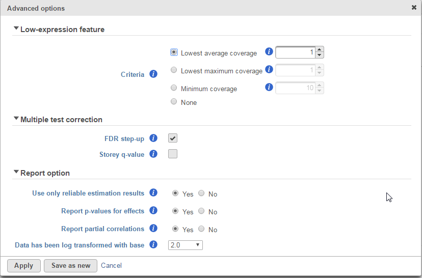
Low-expression feature and Multiple test correction sections are the same as the matching GSA advanced option, see above GSA advanced options
Report option
User only reliable estimation results:
there There are situations when a model estimation procedure does not fail outright, but still encounters some difficulties. In this case, it can even
it can generate p-value and fold change on the comparisons, but they are not reliable, i.e. they can be misleading.
It is recommended that only reliable estimation results should be used, so Therefore, the default of Use only reliable estimation results is set Yes.
Display p-value for effects:
When you choose If set to No,
only only the p-value of comparison will be displayed on the report, the p-value of the factors and interaction terms are not shown in the report table. When you choose Yes in addition to the
comparison's comparison’s p-value, type III p-values are displayed for all the non-random terms in the model.
Report partial correlations: If the model has a numeric factor(s), when choosing Yes, partial correlation coefficient(s) of the numeric factor(s) will be displayed in the result table. When choosing No, partial correlation coefficients are not shown.
Data has been log transformed with base: showing the current scale of the input data on this task.
ANOVA report
Since there is only one model for all features, so there is no pie charts design models and response distribution information. The Gene list table format is the same as the GSA report.
...
This option is only available when Cufflinks quantification node is selected. Detailed implementation information can be found from in the Cuffdiff manual [65].
When the task is selected, the dialog will display all the categorical attributes which have more than one subgroups (Figure 18).
Figure 18: Cuffdiff dialog
| Numbered figure captions | ||||
|---|---|---|---|---|
| ||||
Click on Configure button in the Advanced options to configure normalization method and library types (Figure 19).
Figure 19:
| Numbered figure captions | ||||
|---|---|---|---|---|
| ||||
- Class-fpkm: library size factor is set to 1, no scaling applied to FPKM values
Geometric: FPKM are scaled via the median of the geometric means of the fragment counts across all libraries [
76]. This is the default
optionoption (and is identical to the one used by DESeq)
- Quartile: FPKMs are scaled via the ratio of the 75 quartile fragment counts to the average 75 quartile value across all libraries
...
The report of the cuffdiff task is a table of a feature list with all the comparisons p-valuevalues, q-value and log2 fold-change information for all the comparisons (Figure 20).
| Numbered figure captions | ||
|---|---|---|
|
| |||
- NOTEST: not enough alignments for testing
- LOWDATA: too complex or shallowly sequences
- HIGHDATA: too many fragments in locus
- FAIL: when an ill-conditioned covariance matrix or other numerical exception prevents testing
The table can be downloaded as text a text file when clicking the Download button on the lower-right corner of the table.
...
Overview
Content Tools