Page History
...
Trajectory analysis by Monocle 3 requires data normalisation and preprocessing. We suggest to run the Recommended normalization from the Normalization and scaling section of the toolbox (i.e. normalize by counts per million, add offset of 1, and then log2 transform). According to the Monocle 3 authors, you may want to filter in the top 5,000 genes with the highest variance (2,000 genes for datasets with fewer than 5,000 cells, and 300 genes for datasets with fewer than 1,000 cells) (1). Those number should be used as a guidance for the first-pass analysis and may need to be optimized, depending on the actual analysisproject at hand and the biological question.
Setting up Trajectory Analysis
...
Under the hood, Monocle 3 will project the gene count matrix into the top 50 principal components. Next, the dimensionality reduction will be implemented by UMAP (using default settings of the reduce_dimension command).
Trajectory Analysis Result
Result of running Trajectory analysis in Partek Flow is the Trajectory result data node. Double clicking on the node opens a Data Viewer window with the trajectory plot (Figure xxx1). Cell trajectory graph shows position of each cell (blue dot) with respect to the UMAP coordinates (axes). Cell trajectories (one or more, depending on the data set) are depicted as black lines. Gray circles are trajectory nodes (i.e. cell communities).
...
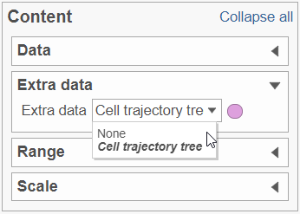
To show / hide cell trajectory tree and trajectory nodes, use the Extra data option on the Content card (Figure xxx2).
| Numbered figure captions | ||||
|---|---|---|---|---|
| ||||
|
...
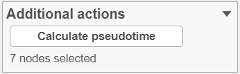
To perform pseudotime analysis, you need to point to the cells at the beginning of the biological process you are interested in. For example, cells at the earliest stage of differentiation sequence. To start, select the root cell nodes (gray circles) by left-click. If the trajectory result consists of more than one trajectory tree, you can specify more than one root node, e.g. one root node per trajectory tree (ctrl & click). If no root node is specified for a tree, that tree will not be included in the pseudotime calculation. Figure xxx 3 shows an example where seven root nodes were identified.
...
Once you have identified all the root nodes, push the Calculate pseudotime button in the Selection panel (Figure xxx4).
| Numbered figure captions | ||||
|---|---|---|---|---|
| ||||
|
...
As a result, the cells will be annotated by pseudotime, using green to red gradient (start and end, respectively) (Figure xxx5). If, for a particular tree, no root node has been specifiedidentified, those cells will be omitted from the pseudotime calculation and will be colored in gray (not shown).
...
| Numbered figure captions | ||||
|---|---|---|---|---|
| ||||
|

As a result of Following pseudotime calculation, three types of cell nodes will become apparent be annotated on the plot (in addition to the intermediate nodes from the previous step).
- Root node (white). Root nodes are start points of the pseudotime and were defined by the user in the previous step (e.g. node 7 in Figure xxx6).
- Branch node (black). Branch nodes indicate where the trajectory tree forks out; i.e. each branch represents a different cell fate or different trajectory (e.g. nodes 1 and 4 in Figure xxx6).
- Leaf (light gray). Leaves correspond to different cell fates / different trajectory outcomes (e.g. nodes 3, 8, and 11 in Figure xxx6). The leaves correspond to cell states of Monocle 2.
...
Overview
Content Tools