Page History
What is Graph-based clustering?
Graph-based clustering is a method for identifying groups of similar cells or samples. It makes no prior assumptions about the clusters in the data. This means the number, size, density, and shape of clusters does not need to be known or assumed prior to clustering. Consequently, graph-based clustering is useful for identifying clustering in complex data sets such as scRNA-seq.
Running Graph-based clustering
We recommend normalizing your data prior to running Graph-based clustering, but the task will run on any counts data node.
...
| Numbered figure captions | ||||
|---|---|---|---|---|
| ||||
|
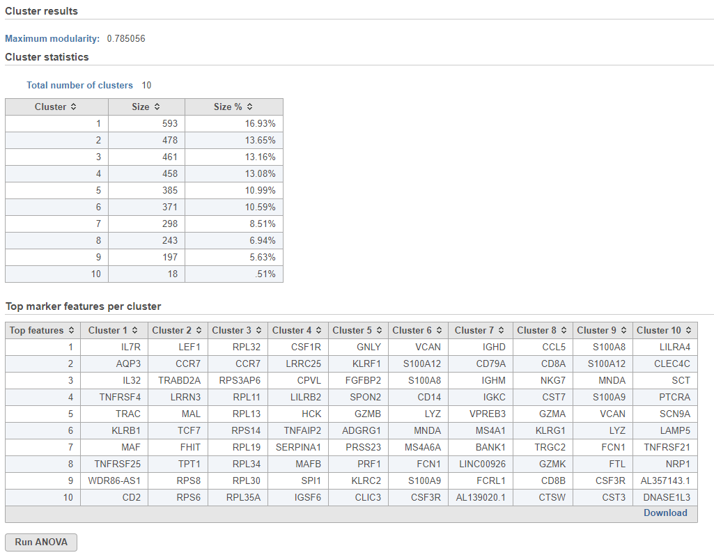
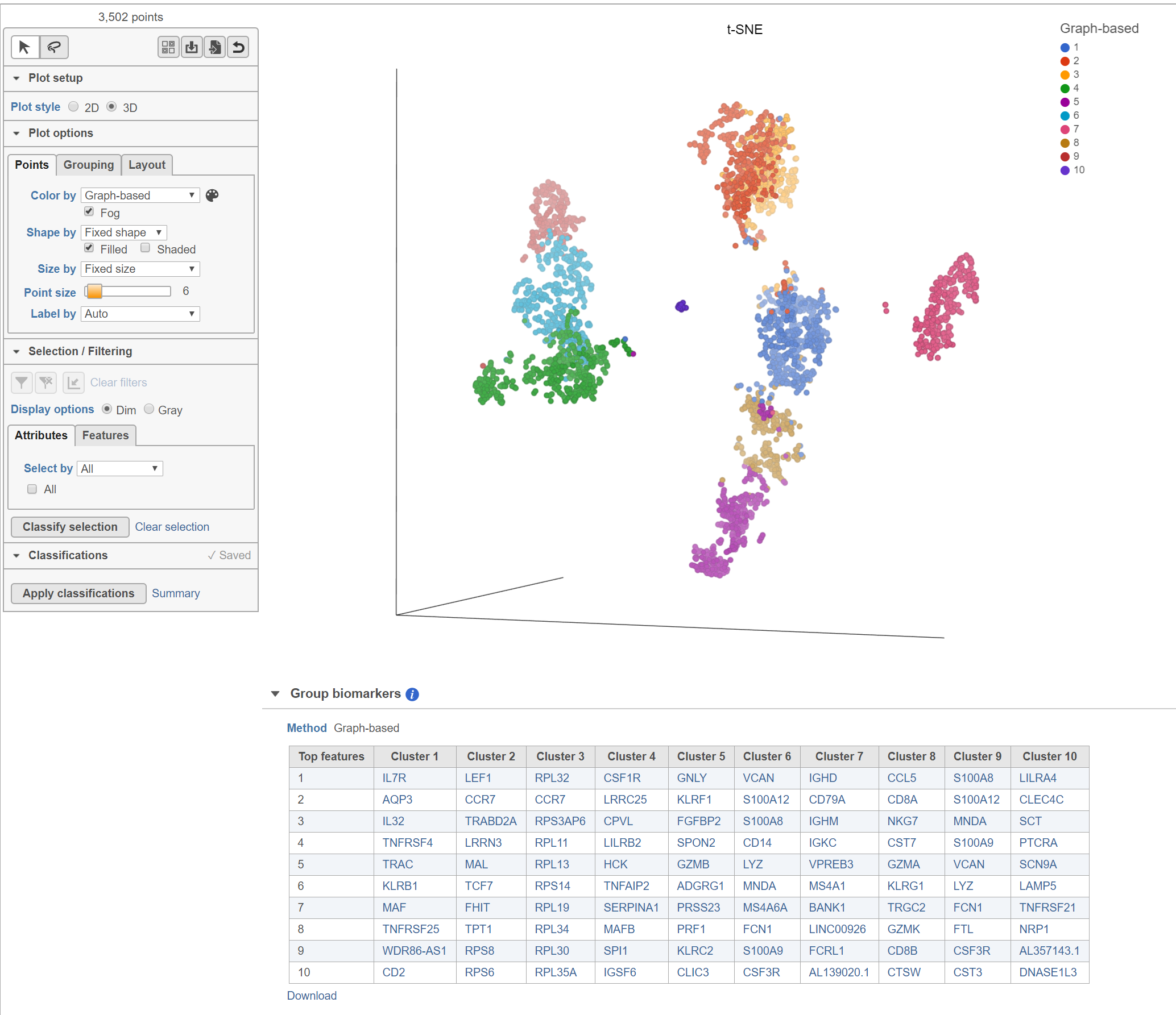
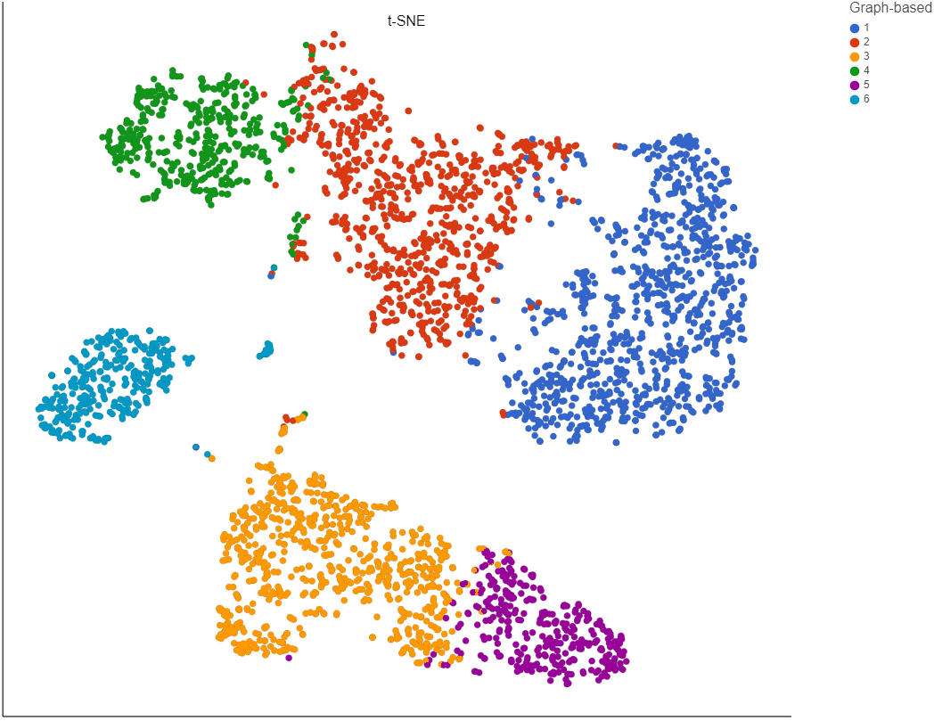
Cluster results
The Maximum modularity is a measure of the quality of the clustering result. Modularity measures how much cells within a cluster are similar to each other and less similar to cells in other clusters. Higher modularity indicates a better result. Optimal modularity is 1, but may not be attainable for the input data.
Cluster statistics
The total number of clusters is listed along with the number and percentage of cells in each cluster.
Top marker features per cluster
Biomarkers for each cluster are calculated using an ANVOA test where each cluster is compared to the other cells in the data set, genes with fold-change > 1.5 are included, and these genes are sorted by ascending p-value (ties broken by greater fold change). The top 10 genes for each cluster are shown in the table. The full ANOVA results can be obtained by clicking the Run ANOVA button, which will generate a Feature list data node.
...
| Numbered figure captions | ||||
|---|---|---|---|---|
| ||||
|
Basic Graph-based clustering parameters
Clustering algorithm
Choose which version of the Louvain clustering algorithm to use. Options are Louvain [1], Louvain with refinement [2], and SLM [3]. The most recent version is Smart Local Moving (SLM). The default is Louvain.
Split cells by sample
Chose whether to run Graph-based clustering on all samples together or on each sample individually.
Checking the box will run Graph-based clustering on each sample individually.
Include features where "Feature type" is
This option appears when there are multiple feature types in the input data node (e.g., CITE-Seq data).
Select Any to run on all features or pick a feature type.
Advanced Graph-based clustering parameters
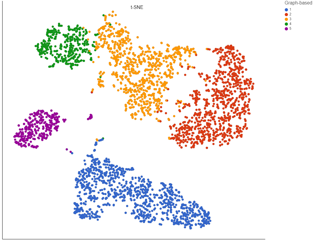
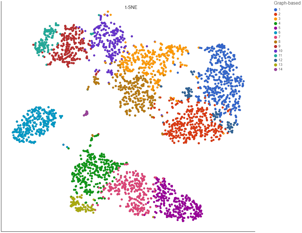
Resolution
To increase the number of clusters, increase the resolution (Figure 3). To decrease the number of clusters, decrease the resolution. Default is 1.
...
| Numbered figure captions | ||||
|---|---|---|---|---|
| ||||
|
Prune parameter
Removes links between pairs of points if their similarity is below the threshold. Larger values lead to a shorter run time, but can result in many singleton clusters. Default is 0.0.
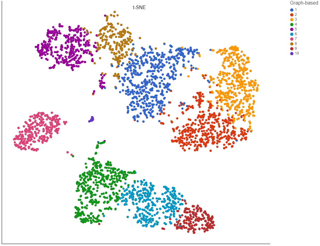
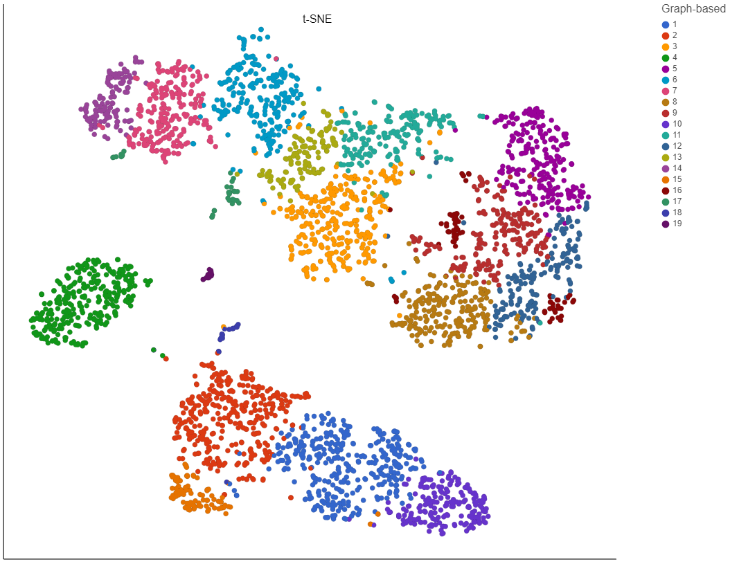
Number of nearest neighbors
Clustering preserves the local structure of the data by focusing on the distances between each point and its k nearest neighbors. The optimal perplexity depends on the size and density of the data. Generally, a larger and/or more dense data set will benefit from a larger number of nearest neighbors. Increasing the number of nearest neighbors will increase the size of clusters and vice versa (Figure 4). Default is 30. The range of possible values is 3 to 100.
...
| Numbered figure captions | ||||
|---|---|---|---|---|
| ||||
|

Scale
This parameter can be used to speed up clustering at the expense of accuracy. Larger scale implies greater accuracy and helps avoid singletons, but takes more time to run. To maximize accuracy, the total count of observations being clustered should be below the product of nearest neighbors and scale. Default is 100,000. The range of possible values is 1 to 100,000.
Modularity function
The modularity function measures the overall quality of clustering. Graph-based clustering amounts to finding a local maximum of the modularity function. Possibilities are Standard [4] and Alternative [5]. Default is Standard.
Number of random starts
The clustering result depends on the order observations are considered. Each random start corresponds to a different order and result. A larger number of random starts can deliver a better result because the result with the highest quality (modularity) out of all of the random starts is chosen. Increasing the number of random starts will increase the run time. The range of possible values is 3 to 1,000. The default is 100.
Random seed
The random seed is used in the random starts portion of the algorithm. Using a different seed might give a better result. Use the same random seed to reproduce results. Default is 0.
Number of iterations per random start
To maximize modularity, clustering proceeds iteratively by moving individual points, clusters, or subsets of points within clusters. A larger number of iterations can give better results, but will take longer to run. Default is 10.
Minimal cluster size
Clusters smaller than the minimal cluster size value will be merged with a nearby cluster unless they are completely isolated. To avoid isolation, set the prune parameter to zero (default) and the scale parameter to the maximum (default). Default is 1.
Sequential random starts
Enable this option to use the slower sequential ordering of random starts. Default is disabled.
Nearest Neighbor Type
Different methods for determining nearest neighbors. The K nearest neighbors (K-NN) algorithm is the standard. The NN-Descent algorithm is used by UMAP and is an alternative. Default is K-NN.
Distance metric
If NN-Descent is chosen for Nearest Neighbor Type, the metric to use when determining distance between data points in high dimensional space can be set. Options are Euclidean, Manhattan, Chebyshev, Canberra, Bray Curtis, and Cosine. Default is Euclidean.
PCA: Number of principal components
Graph-based clustering uses principal components as its input. The number of principal components to use is set here.
We recommend using the PCA task to determine the optimal number of principal components for your data. Default is 100.
PCA: Features contribute
Options are equally or by variance. Feature values can be standardized prior to PCA so that the contribution of each feature does not depend on its variance. To standardize, choose equally. To take variance into account and focus on the most variable features, choose by variance. Default is by variance.
Normalization: Log transform data
You can choose to log transform the data prior to running PCA as part of Graph-based clustering. Default is disabled.
Normalization: Log base
If you are normalizing the data, choose a log base. Default is 2 when Log transform data is enabled.
Normalization: Log offset
If you are normalizing the data, choose an offset. Default is 1 when Log transform data is enabled.
References
[1] Blondel, V. D., Guillaume, J. L., Lambiotte, R., & Lefebvre, E. (2008). Fast unfolding of communities in large networks. Journal of statistical mechanics: theory and experiment, 2008(10), P10008.
...
Overview
Content Tools