Page History
Raw read counts are generated after quantification for each feature on all samples. These read counts need to be normalized prior to differential expression detection to ensure that samples are comparable.
This chapter covers the implementation of each normalization method. The Normalize counts option is available on the When a sample or a group of sample serves as control baseline in the experiment design, other samples can be normalized by subtracting or divided by the baseline sample(s), e.g. in PCR data to obtain delta delta CT values.
The Normalize to baseline option is available at the Normalization and Scaling section in the context-sensitive menu (Figure 1) upon selection of any quantified output data node or an imported count matrix:
- Gene counts
- Transcript counts
- MicroRNA counts
- Cufflinks quantification
- Quantification
containing matrix of measurements of observations (e.g. samples) on features (e.g genes).
...
| Numbered figure captions | ||||
|---|---|---|---|---|
| ||||
|

The format of the output is the same as the input data format, the node is called Normalized counts. This data node can be selected and normalized further using the same task.
Selecting Methods
Select whether you want your data normalized on a per sample or per feature basis (Figure 2). Some transformations are performed on each value independently of others e.g. log transformation, and you will get an identical result regardless of your choice.
| Numbered figure captions | ||||
|---|---|---|---|---|
| ||||
|
The following normalization methods will generate different results depending on whether the transformation was performed on samples or on features:
- Divided by mean, median, Q1, Q3, std dev, sum
- Subtract mean, median, Q1, Q3, std dev, sum
- Quantile normalization
Note that each task can only perform normalization on samples or features. If you wish to perform both transformations, run two normalization tasks successively. To normalize the data, click on a method from the left panel, then drag and drop the method to the right panel. Add all normalization methods you wish to perform. Alternatively, you can click on the green plus button () on each method to add it. Multiple methods can be added to the right panel and they will be processed in the order they are listed. You can change the order of methods by dragging each method up or down. To remove a method from the Normalization order panel, click the minus button (
![]() ) to the right of the method. Click Finish, when you are done choosing the normalization methods you have chosen.
) to the right of the method. Click Finish, when you are done choosing the normalization methods you have chosen.
Recommended Methods
For some data nodes, recommended methods are available:
- Data nodes resulting from Quantify to annotation model (Partek E/M) or Quantify to reference (Partek E/M) are raw read counts, the recommendation is Total Count, Add 0.0001
- Cufflinks quantification data node output FPKM normalized read counts, the recommendation is Add 0.0001
| |
|
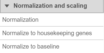
There are three options to choose baseline samples:
- use all samples
- use group
- use matched pairs
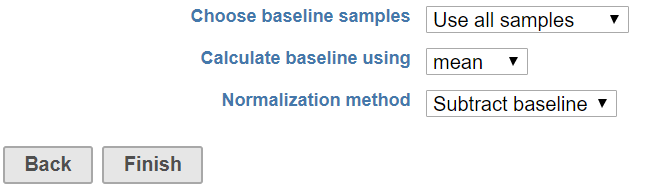
Use all samples to create baseline
To normalize data to all the samples, choose to use mean or median of all samples for each feature, and select subtract baseline or ratio to baseline in the normalization method (Figure 2), click Finish.
...
- Normalize the reads by the length of feature, it generate reads per kilobase
RPKsf = Xsf / Lf; - Sum up all the RPKsf in a sample
PRKs = ∑Ff=1 FRPKsf - Generate a scaling factor for each sample by normalizing the PRK of the sample to the sum PRK of all the samples
 ,
,
where TR is the total reads across all samples - Divide raw reads by the scaling factor to get TPM
TXsf = Xsf/Ks
- Normalize the reads by the length of feature, it generate reads per kilobase
- Upper quartile
- The method is exactly the same as the LIMMA package [7].
The following is the simple summarization of the calculation:
- Remove all the features that have 0 reads in all samples.
- Calculate the effective library size per sample: effective library size = (raw library size (in millions))*((upper quartile for a particular sample)/ (geometric mean of upper quartiles in all the samples))
- Get the normalized counts by dividing the raw counts per feature by the effective library size (for the respective sample)
Normalization Report
The Normalization report includes the Normalization methods used, a Feature distribution table, Box-whisker plots of the Expression signal before and after normalization, and Sample histogram charts before and after normalization. Note that all visualizations are disabled for results with more than 30 samples.
Normalization methods
A summary of the normalization methods performed. They are listed by the order they were performed.
Feature distribution table
A table that presents descriptive statistics on each sample, the last row is the grand statistics across all samples (Figure 4).
| Numbered figure captions | ||||
|---|---|---|---|---|
| ||||
|

Expression signal
These box-whisker plots show the expression signal distribution for each sample before and after normalization. When you mouse over on each bar in the plot, a balloon would show detailed percentile information (Figure 5).
| Numbered figure captions | ||||
|---|---|---|---|---|
| ||||
|

Sample histogram
A histogram is displayed for data before and after it is normalized. Each line is a sample, where the X axis is the range of the data in the node and the Y-axis is the frequency of the value within the range. When you mouse over a circle which represent a center of an interval, detailed information will appear in a balloon (Figure 6). It includes:
- The sample name.
- The range of the interval, “[ “represent inclusive, “)” represent exclusive.
- The frequency value within the interval
| Numbered figure captions | ||||
|---|---|---|---|---|
| ||||
|

References
- Bolstad BM, Irizarry RA, Astrand M, Speed, TP. A Comparison of Normalization Methods for High Density Oligonucleotide Array Data Based on Bias and Variance. Bioinformatics. 2003; 19(2): 185-193.
- Mortazavi A, Williams BA, McCue K, Schaeffer L, Wold B. Mapping and quantifying mammalian transcriptomes by RNA-Seq. Nat Methods. 2008; 5(7): 621–628.
- Bullard JH, Purdom E, Hansen KD, Dudoit S. Evaluation of statistical methods for normalization and differential expression in mRNA-Seq experiments. BMC Bioinformatics. 2010; 11: 94.
- Robinson MD, Oshlack A. A scaling normalization method for differential expression analysis of RNA-seq data. Genome Biol. 2010; 11: R25.
- Dillies MA, Rau A, Aubert J et al. A comprehensive evaluation of normalization methods for Illumina high-throughput RNA sequencing data analysis. Brief Bioinform. 2013; 14(6): 671-83.
- Wagner GP, Kin K, Lynch VJ. Measurement of mRNA abundance using RNA-seq data. Theory Biosci. 2012; 131(4): 281-5.
- Ritchie ME, Phipson B, Wu D et al. Limma powers differential expression analyses for RNA-sequencing and microarray studies. Nucleic Acids Res. 2015; 43(15):e97.
...
| Numbered figure captions | ||||
|---|---|---|---|---|
| ||||
|

Normalization Methods
Below is the notation that will be used to explain each method:
| Symbol | Meaning |
|---|---|
| S | Sample (or cell for single cell data node) |
| F | Feature |
| Xsf | Value of sample S from feature F (if normalization is performed on a quantification data node, this would be the raw read counts) |
| TXsf | transformed value of Xsf |
| C | Constant value |
| b | Base of log |
- Absolute value
TXsf = | Xsf | - Add
TXsf = Xsf + C
a constant value C needs to be specified - Antilog
TXsf = bxsf
A log base value b needs to be specified from the drop-down list; any positive number can be specified when Custom value is chosen - CLR (centered log ratio)
TXsf =ln((Xsf +1)/geom (Xsf +1) +1)
geom is geometric mean of either observation or feature. We recommend to perform this normalization on observation for CITE seq data.
...
| |||
|
Use a group of sample to create baseline
When there are a subset of samples serve as baseline in the experiment, choose use group as baseline samples. The specific group needs be specified from the sample attributes (Figure 3)
| Numbered figure captions | ||||
|---|---|---|---|---|
| ||||
|
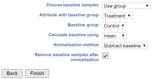
Choose this option, select the attribute containing the baseline group information, e.g. Treatment in this example, the samples labeled as Control will be used as baseline. After normalization, the control sample can be filtered out in the report by selecting Remove baseline samples after normalization check button
Use matched pairs
In a paired experiment design, when normalized one sample to its own control – typically there is only one sample serve as a control to its pair (Figure 4), an attribute on the pair information should be specified in addition to baseline group attribute.
| Numbered figure captions | ||||
|---|---|---|---|---|
| ||||
|
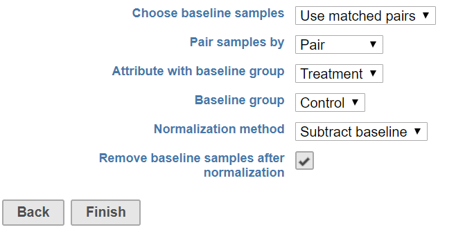
Choose the attribute containing information to pair the samples, and select the attribute with control sample information. After normalization, the control sample should be either 0 or 1 depending all the normalization method chosen, so we highly recommend remove control samples in the report.
| Additional assistance |
|---|
|
| Rate Macro | ||
|---|---|---|
|
Overview
Content Tools